Download
1 / 48
480 likes | 716 Vues
Index Velocity Best Practices ADVMs. Victor Levesque USGS FISC - Tampa. Overview. Configuring SonTek ADVMs Servicing SonTek ADVMs Use of the Internal Data Recorder Beam Checks Data to Transmit and Store Quality Assurance of Data Common Problems. Configuring the Instrument.

E N D
Index Velocity Best PracticesADVMs Victor Levesque USGS FISC - Tampa
Overview • Configuring SonTek ADVMs • Servicing SonTek ADVMs • Use of the Internal Data Recorder • Beam Checks • Data to Transmit and Store • Quality Assurance of Data • Common Problems
Configuring the Instrument • Use SonUtils (v4.20) • Initial Setup • Use Theoretical Flow Disturbance Estimate for Cell Begin and Blanking Distance • Use Beam Check Signal Intensities for Cell End • Refine the Setup • Use multi-cell velocity data to verify and check for flow disturbance for Cell Begin • Use multi-cell velocity data to verify and check for appropriate Cell End
b = c(dx)0.5 b -- lateral distance from pier centerline to edge of wake zone d -- pier width x -- distance to upstream face of pier c -- factor for pier shape 0.62 - round nosed 0.81 – rectangular nosed x d b Configuring the Instrument Theoretical Flow Disturbance for Cell Begin and possibly Cell End • Structure turbulence must be considered when establishing start of sample volume
Configuring the Instrument Cell Begin Marker Initially Use Beam Check for Setting Cell End Remember that scatterers in the water will change over time affecting signal strength. Cell End Marker Instrument Noise Floor Marker Decay Curve
Configuring the Instrument Use SonUtils and SI units (meters) • Set Blanking Distance (BD) = Cell Begin (CB) • Enable Profiling Mode (ProfilingMode Yes) • Choose Cell Size (CS) and Number of Cells (Ncells) to at least equal Cell End (CE) • Example: CB = 1 meter => BD = 1 meter CE = 11 meters based on Beam Check CS = 1 meter and Ncells = 10 So multi-cell data starts at 1 meter and ends at CS * Ncells + BD = 1 * 10 + 1 = 11 meters
Configuring the Instrument Special Considerations for XR and SW • Enable Dynamic Boundary Adjustment(DynamicBoundaryAdjustment Yes) • XR uses non-vented pressure sensor to set CE • Pressure sensor is affected by atmospheric pressure changes and temperature changes. Pressure sensor can drift or fail over time • SW uses vertical beam level (distance) to set CE Note: CE = Cell End
Configuring the Instrument • Enable Power Ping (PowerPing Yes) • 1.5 MHz and 3 MHz systems What about Sample Interval (SI) and Averaging Interval (AI)?
Configuring the Instrument • Averaging Interval (AI) • What do you want to measure and what are the flow conditions? • Rapidly changing flow may require shorter averaging interval • General rule Increased averaging time => lower velocity standard deviation • Recommend 60 seconds AI and SI during discharge measurements
Configuring the Instrument • Sampling Interval (SI) • 900 seconds maximum for tidally affected sites • Could be as short as 60 seconds • SI >= AI
Configuring the Instrument • Example: Steady state stream with backwater affects • AI = 600 seconds • SI = 900 seconds • Note: Actual settings may vary • Remember that if stream is flashy,shorter AI and SI may be requiredto measure the peak • Make sure you have enough battery and solar capacity to meet power demands • May or may not change averaging interval during discharge measurements
Configuring the Instrument • Example: Tidally affected flow • AI = 60 - 780 seconds • SI = 60 to 900 seconds • Set AI = SI = 60 seconds during discharge measurements • Data times are extremely important
Configuring the Instrument • Example: Unsteady flow due to seiche in small tributary of a larger river • What are you trying to measure? Daily flow? Short term fluctuations? • AI = 60 to 780 seconds • SI = 60 to 900 seconds • Set AI = SI = 60 seconds during discharge measurements • Data times are extremely important
Configuring the Instrument • Discharge measurements • AI = 60 seconds • SI = 60 seconds • Set StartTime (ST) hh:mm:ss • Set StartDate (SD) YYYY/MM/DD • Record Internally (disable SDI12 communication) • Deploy (leave Molex plug connected)
Evaluate the Configuration Use Multi-cell data to evaluate flow disturbance
Evaluating the Configuration More obvious way to see flow disturbance is with plot of index velocity and mean velocity from measurements.
Servicing ADVMs with SonUtils • Record a beam check (50 pings minimum) • Example: stationID_YYYYMMDD.bmc • Download ADVM internal data • Open a log file (click File in menu bar, open log file) • Example: stationID_YYYYMMDD.log • Record instrument and watch date and time before changing (use a form) • Change AI and SI if necessary • Change StartDate (SD) and StartTime (ST) • Deploy ADVM • Close log file
Use the Internal Recorder • Valuable data set • Use ViewArgonaut for data review • Select Processing • Open an Argonaut file • Look for anomalies in the data • Check all available parameters • Check internal beam checks (DIAG) tab on menu bar • Look at signal strengths for each beam • Look at multi-cell velocity data
Velocity and SNR • Added QA • Additional backup source • Added understanding of site hydraulics over time XYZ components
…Ability To See Different Velocity Components • Problem identified as Beam 2 issue Beam components
Using the Internal Recorder • Review the data after every site visit • Range-averaged cell velocity (X,Y, and Z) • Compare multi-cell to range-averaged velocity • Signal amplitude and instrument noise • ADVM temperature • Everything else • Plot questionable record and add to review folder • Recommend storing internal data in ADAPS
Beam Checks • Record every site visit • Record 50 pings minimum • Average the pings together • Transfer and store on WSC server
Beam Checks Cell Begin Marker Initially Use Beam Check for Setting Cell End Remember that scatterers in the water will change over time affecting signal strength. Cell End Marker Instrument Noise Floor Marker Decay Curve
Obstructions in the sample volume Beam Checks—What To Look For
Dead beam Beam Checks—What To Look For
Possible reflection off of the bed or surface Beam Checks—What To Look For
Hardware issues—high noise floor Beam Checks—What To Look For
Fouled transducers Beam Checks—What To Look For
Data to Transmit and Store • Minimum • ADVM Temperature • Cell End • X velocity • Y velocity • Average signal to noise ration • Ideally in addition to above data • Mean pressure if applicable • Level if applicable • Archive all Argonaut internal dataaccording to WSC data archival plan • 00055 Stream velocity, feet per second • 72149 Stream velocity, meters per second • 72168 Stream velocity, tidally filtered, feet per second • 72169 Stream velocity, tidally filtered, meters per second • 99237 Acoustic Doppler Velocity Meter signal to noise ratio • 99238 Location of Acoustic Doppler Velocity Meter cell end, feet • 99239 Acoustic Doppler Velocity Meter standard deviation, data element specified in data descriptor • 99240 Acoustic Doppler Velocity Meter standard error of velocity, feet per second • 99241 Location of Acoustic Doppler Velocity Meter cell end, meters • 99242 Acoustic Doppler Velocity Meter standard error of velocity, centimeters per second • 99968 Acoustic signal strength, units specified in data descriptor
Common Problems • Beam Check hangs during recording • Communication to internal recorder fails • PowerPing disabled • No multi-cell data measured • Argonaut-XR pressure sensor drift or failure • Beam fouling – No beam checks • Sensor not level • Cell End set too long • Cell Begin set too short • Internal clock never checked or reset • Internal recorder data not reviewed
Common Problems • Poor Index-to-Mean Velocity Relation • Stage affected velocity profile • Try multiple-linear regression • Poor site selection • Streambed instability • Unstable horizontal flow distribution • Improper instrument selection or configuration • XR or SW instead of SL • Cell begin and cell end not set properly
Flood tide Ebb tide Tomoka River at Ormond Beach Gage
Second SonTek SL SonTek XR Original SonTek SL
Site Selection Keep in mind • Fundamental question– will we be able to index the mean channel velocity over the range of flows at the selected site? • Keys for a successful site • Stable stream bed • Well mixed flow will have long-term stable vertical velocity profiles and horizontal flow distributions • Stable profiles and distributions allow us to create index-velocity ratings
Reconnaissance of Potential Sites • Other Tools • Temporary ADVM • Aerial Photos, Charts, and Maps • Flow conditions recon with an ADCP • Velocity profiles • Depths • Shoals • Structures
Common Problems • Wrong firmware on instrument • Use v11.8 for all Argonaut-SL, SW, and XR • Contact USGS Hydroacoustics • Wrong software • SonUtils v4.20 • ViewArgonaut v3.62 • Poor Equipment Mounts • Allow pitch and roll adjustment • Minimize dissimilar metals • Allow sensor to be replaced in exact position
/flalssr003/ ds measurements (discharge and velocity) ds.archive WY2003 WY2004 WY2005 data logger (work/temporary) sta # 02243960 sta # sta # data logger etc. etc. adcp argonaut flowtracker aquacalc (station #_mmddyy) archive WY2003 WY2004 02243960_040602.ckg 02243960_040602.bmc 02243960_040602.log 02243960_040602.arg (See note below for file type explanation.) 02243960_040602_000w.000 02243960_040602_000w.001 02243960_040602_000r.001 02243960_.wrc 2421.020406152212.txt .aqu 02243960.237.dis 02243960.237.wad02243960.237.ctl 02243960.237.dat 02243960.237.sum02243960.237.ckg (station #. measurement #) Document and Archive Everything