Download
1 / 28
280 likes | 486 Vues
Welcome to... the Crash Course Probability Theory. Marco Loog. Outline. Probability Syntax Axioms Prior & conditional probability Inference Independence Bayes’ Rule. First a Bit Uncertainty. Let action A[t] = leave for airport t minutes before flight Will A[t] get me there on time?

E N D
Welcome to... the Crash Course Probability Theory Marco Loog
Outline • Probability • Syntax • Axioms • Prior & conditional probability • Inference • Independence • Bayes’ Rule
First a Bit Uncertainty • Let action A[t] = leave for airport t minutes before flight • Will A[t] get me there on time? • Problems • Partial observability [road state, other drivers’ plans, etc.] • Noisy sensors [traffic reports] • Uncertainty in action outcomes [flat tire, etc.] • Immense complexity of modeling and predicting traffic
Several Methods for Handling Uncertainty • Probability is only one of them... • But probably the one to prefer • Model agent’s degree of belief • Given the available evidence • A[25] will get me there on time with probability 0.04
Probability • Probabilistic assertions summarize effects of • Laziness : failure to enumerate exceptions, qualifications, etc. • Ignorance : lack of relevant facts, initial conditions, etc.
Subjective Probability • Probabilities relate propositions to agent’s own state of knowledge • E.g. P(A[25] | no reported accidents) = 0.06 • Probabilities of propositions change with new evidence • E.g. P(A[25] | no reported accidents, 5 a.m.) = 0.15
Making Decisions under Uncertainty • Suppose I believe the following • P(A[25] gets me there on time | …) = 0.04 • P(A[90] gets me there on time | …) = 0.70 • P(A[120] gets me there on time | …) = 0.95 • P(A[1440] gets me there on time | …) = 0.9999 • Which action to choose? • Depends on my preferences for missing flight vs. time spent waiting, etc. • Utility theory is used to represent and infer preferences • Decision theory = probability theory + utility theory
Syntax • Basic element : random variable • Referring to ‘part’ of world whose ‘status’ is initially unknown • Boolean random variable • Cavity [do I have a cavity?] • Discrete random variables • Weather is one of <sunny,rainy,cloudy,snow> • Elementary proposition constructed by assignment of value to random variable • Weather = sunny, Cavity = false • Complex propositions formed from elementary propositions and standard logical connectives • Weather = sunny Cavity = false
Syntax • Atomic events : complete specification of state of the world about which the agent is uncertain • E.g. if the world consists of only two Boolean variables Cavity and Toothache, then there are 4 distinct atomic events : • Cavity = false Toothache = false • Cavity = false Toothache = true • Cavity = true Toothache = false • Cavity = true Toothache = true • These are mutually exclusive & exhaustive
Axioms of Probability • For any propositions A, B • 0 ≤ P(A) ≤ 1 • P(true) = 1 and P(false) = 0 • P(A B) = P(A) + P(B) - P(AB)
Prior Probability • Prior or unconditional probabilities of propositions • P(Cavity = true) = 0.1 and P(Weather = sunny) = 0.72 correspond to belief prior to arrival of any (new) evidence • Probability distribution gives values for all possible assignments • P(Weather) = <0.72,0.1,0.08,0.1> [normalized, i.e., sums to 1]
Prior Probability • Joint probability distribution for a set of random variables gives the probability of every atomic event on those random variables • P(Weather,Cavity) = 4 × 2 matrix of values • Weather = sunny rainy cloudy snow • Cavity = true 0.144 0.02 0.016 0.02 • Cavity = false 0.576 0.08 0.064 0.08 • Every question about a domain can be answered by the joint distribution
Conditional Probability • Conditional or posterior probabilities • E.g. P(cavity | toothache) = 0.8, i.e., given that toothache is all I know • If we know more, e.g. cavity is also given, then we have • P(cavity | toothache,cavity) = 1
Conditional Probability • New evidence may be irrelevant, allowing simplification, e.g. • P(cavity | toothache, sunny) = P(cavity | toothache) = 0.8 • This kind of inference, sanctioned by domain knowledge, is crucial
Conditional Probability • Definition of conditional probability • P(a | b) = P(a b) / P(b) if P(b) > 0 • Product rule gives an alternative formulation • P(a b) = P(a | b) P(b) = P(b | a) P(a)
Conditional Probability • General version holds for whole distributions • P(Weather,Cavity) = P(Weather | Cavity) P(Cavity) • Chain rule is derived by successive application of product rule • P(X1, …,Xn) = P(X1,...,Xn-1) P(Xn | X1,...,Xn-1) = P(X1,...,Xn-2) P(Xn-1 | X1,...,Xn-2) P(Xn | X1,...,Xn-1) = … = ∏i P(Xi | X1, … ,Xi-1)
Marginalization & Conditioning • General rule given by conditioning : • P(X | d) = ∑i P(X, hi | d) = ∑i P(X | d, hi) P(hi | d) = ∑i P(X | hi) P(hi | d) • Without the condition on d, it is called marginalization
Inference by Enumeration • Start with the joint probability distribution • For any proposition φ, sum the atomic events where it is true : P(φ) = Σω:ω╞φ P(ω)
Inference by Enumeration • Start with the joint probability distribution • For any proposition φ, sum the atomic events where it is true : P(φ) = Σω:ω╞φ P(ω) • P(toothache) = 0.108 + 0.012 + 0.016 + 0.064 = 0.2
Inference by Enumeration • Start with the joint probability distribution • For any proposition φ, sum the atomic events where it is true : P(φ) = Σω:ω╞φ P(ω) • P(toothache cavity) = 0.2 + 0.08 = 0.28
Inference by Enumeration • Can also do conditional probabilities • P(cavity | toothache) = P(cavity toothache) P(toothache) = 0.016+0.064 0.108 + 0.012 + 0.016 + 0.064 = 0.4
Inference by Enumeration • Obvious problems • Worst-case time complexity O(dn) where d is the largest arity • Space complexity O(dn) to store the joint distribution • How to find the numbers for O(dn) entries?
Independence • A and B are independent iff P(A|B)=P(A) or P(B|A)=P(B) or P(A,B)=P(A)P(B) • P(Toothache, Cavity, Weather)= P(Toothache, Cavity) P(Weather) • Independent coin tosses • Absolute independence powerful but rare • Dentistry is a large field with hundreds of variables, none of which are independent What to do?
Conditional Independence • P(Toothache, Cavity, Catch) has 23 – 1 = 7 independent entries • If I have a cavity, the probability that the probe catches in it doesn’t depend on whether I have a toothache so P(catch | toothache,cavity) = P(catch | cavity) • Similarly : P(catch | toothache,cavity) = P(catch | cavity) • Catch conditionally independent of Toothache given Cavity • P(Catch | Toothache,Cavity) = P(Catch | Cavity) • Equivalent statements are • P(Toothache | Catch, Cavity) = P(Toothache | Cavity) • P(Toothache, Catch | Cavity) = P(Toothache | Cavity) P(Catch | Cavity)
Conditional Independence • In most cases, the use of conditional independence reduces the size of the representation of the joint distribution from exponential in n to linear in n • Conditional independence is our most basic and robust form of knowledge about uncertain environments
Bayes’ Rule • Product rule P(ab) = P(a|b)P(b) = P(b|a)P(a) Bayes’ rule : P(a|b) = P(b|a)P(a)/P(b) • In distributional form P(Y|X) = P(X|Y)P(Y)/P(X) = αP(X|Y)P(Y) • Useful for assessing diagnostic probability from causal probability • P(Cause|Effect) = P(Effect|Cause) P(Cause) / P(Effect)
Bayes’ Rule and Conditional Independence • P(Cavity | toothache catch) • = αP(toothache catch | Cavity) P(Cavity) • = αP(toothache | Cavity) P(catch | Cavity) P(Cavity) • This is an example of a naive Bayes model • P(Cause,Effect[1], … ,Effect[n]) = P(Cause) ∏iP(Effect[i]|Cause) • Total number of parameters is linear in n
Summary • Probability is a rigorous formalism for uncertain knowledge • Joint probability distribution specifies probability of every atomic event • Queries can be answered by summing over atomic events • For nontrivial domains, we must find a way to reduce the joint size • Independence and conditional independence provide certain tools for it