Download
1 / 25
260 likes | 269 Vues
ECE 472/572 - Digital Image Processing. Lecture 6 – Geometric and Radiometric Transformation 09/27/11. Introduction Image format (vector vs. bitmap) IP vs. CV vs. CG HLIP vs. LLIP Image acquisition Perception Structure of human eye Brightness adaptation and Discrimination

E N D
ECE 472/572 - Digital Image Processing Lecture 6 – Geometric and Radiometric Transformation 09/27/11
Introduction Image format (vector vs. bitmap) IP vs. CV vs. CG HLIP vs. LLIP Image acquisition Perception Structure of human eye Brightness adaptation and Discrimination Image resolution Image enhancement Enhancement vs. restoration Spatial domain methods Point-based methods Log trans. vs. Power-law Contrast stretching vs. HE Gray-level vs. Bit plane slicing Image averaging (principle) Mask-based methods - spatial filter Smoothing vs. Sharpening filter Linear vs. Non-linear filter Smoothing (average vs. Gaussian vs. median) Sharpening (UM vs. 1st vs. 2nd derivatives) Frequency domain methods Understanding Fourier transform Implementation in the frequency domain Low-pass filters vs. high-pass filters vs. homomorphic filter Geometric correction Affine vs. Perspective transformation Homogeneous coordinates Inverse vs. forward transform Composite transformation General transformation Model distortion with polynomial Least square solution Roadmap
Questions • Affine transformation vs. Perspective transformation • Forward transformation vs. Inverse transformation • Composite transformation vs. Sequential transformation • Homogeneous coordinate • General geometric transformations
Usage • Image correction • Color interpolation • Forensic analysis • Entertainment effect http://www.mpi-sb.mpg.de/resources/FAM/demos.html http://w3.impa.br/~morph/
Affine transformations • Preserve lines and parallel lines • Homogeneous coordinates • General form • Special matrices • R: rotation, S: scaling, T: translation, H: shear
Composite vs. Sequential transformation T S H R Transformed Image (g(u, v)) Original Image (f(x,y))
Forward vs. Inverse transforms Inverse transform Forward transform
Examples - Shear hx = 0.2 hx = hy = 0.2 hy = 0.2
Examples – Translation + Rotation theta = PI/4 tx = -140, ty = 60 theta = PI/4
Perspective transformation • Preserve parallel lines only when they are parallel to the projection plane. Otherwise, lines converge to a vanishing point • General form
Determine the coefficients 8 unknowns, 4-point least squares (0,0) (0,255) (0,0) (0,255) (255,0) (255,255) (255,0) (511,511)
General approaches • Find tiepoints • Spatial transformation
Example – CCD butting misalignment greater than 50 micron x-ray sensitive scintillator fiber optics CCD array 1242 x 1152
Sources of distortions • defects in the production of fiber-optic tapers • imperfect compression and cutting • different light transfer efficiency across the whole surface
Geometric correction map close control point approximation interpolation map exactly
Spatial transformation • Bilinear equation • n-th degree polynomial • Use information from tiepoints to solve coefficients • Exact solution • Least square solution
How is it applied? • Step 1: Choose a set of tie points • (xi,yi): coordinates of tie points in the original (or distorted) image • (ui,vi): coordinates of tie points in the corrected image • Step 2: Decide on which degree of polynomial to use to model the inverse of the distortion, e.g., • Step 3: Solve the coefficients of the polynomial using least-squares approach • Step 4: Use the derived polynomial model to correct the entire original image For each (u,v) in the corrected image, find the corresponding (x,y) in the original image and use its intensity as the intensity at (u,v).
Example – Geometric correction • Geometric correction of images from butted CCD arrays
Example - Color correction Tiepoints are colors (R, G, B), instead of spatial coordinates
Image warping • Two-pass mesh warping by Douglas Smythe • Reference: G. Wolberg, Digital Image Warping, 1990
Example 1 From Joey Howell and Cory McKay, ECE472, Fall 2000
Example 2 From Adam Miller, Truman Bonds, Randal Waldrop, ECE472, Fall 2000