Download
1 / 27
290 likes | 746 Vues
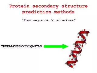
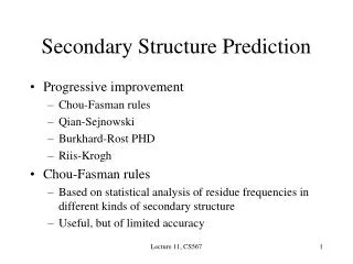
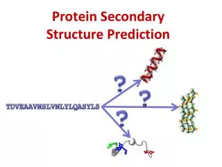
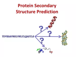
Protein Secondary Structure Prediction. G P S Raghava. Protein Structure Prediction. Importance What is secondary structure Assignment of secondary structure (SS) Type of SS prediction methods Description of various methods Role of multiple sequence alignment/profiles How to use.

E N D
Protein Secondary Structure Prediction G P S Raghava
Protein Structure Prediction • Importance • What is secondary structure • Assignment of secondary structure (SS) • Type of SS prediction methods • Description of various methods • Role of multiple sequence alignment/profiles • How to use
Assignment of Secondary Structure • Program • DSSP (Sander Group) • Stride (Argos Group) • Pcurve • DSSP • 3 helix states (I=3,4,5 ) • 2 Sheets (isolated and extended) • Irregular Regions
dssp • The DSSP program defines secondary structure, geometrical features and solvent exposure of proteins, given atomic coordinates in Protein Data Bank format • Usage: dssp [-na] [-v] pdb_file [dssp_file] • Output : 24 26 E H < S+ 0 0 132 25 27 R H < S+ 0 0 125 26 28 N < 0 0 41 27 29 K 0 0 197 28 ! 0 0 0 29 34 C 0 0 73 30 35 I E -cd 58 89B 9 31 36 L E -cd 59 90B 2 32 37 V E -cd 60 91B 0 33 38 G E -cd 61 92B 0
Automatic assignment programs • DSSP ( http://www.cmbi.kun.nl/gv/dssp/ ) • STRIDE ( http://www.hgmp.mrc.ac.uk/Registered/Option/stride.html ) # RESIDUE AA STRUCTURE BP1 BP2 ACC N-H-->O O-->H-N N-H-->O O-->H-N TCO KAPPA ALPHA PHI PSI X-CA Y-CA Z-CA 1 4 A E 0 0 205 0, 0.0 2,-0.3 0, 0.0 0, 0.0 0.000 360.0 360.0 360.0 113.5 5.7 42.2 25.1 2 5 A H - 0 0 127 2, 0.0 2,-0.4 21, 0.0 21, 0.0 -0.987 360.0-152.8-149.1 154.0 9.4 41.3 24.7 3 6 A V - 0 0 66 -2,-0.3 21,-2.6 2, 0.0 2,-0.5 -0.995 4.6-170.2-134.3 126.3 11.5 38.4 23.5 4 7 A I E -A 23 0A 106 -2,-0.4 2,-0.4 19,-0.2 19,-0.2 -0.976 13.9-170.8-114.8 126.6 15.0 37.6 24.5 5 8 A I E -A 22 0A 74 17,-2.8 17,-2.8 -2,-0.5 2,-0.9 -0.972 20.8-158.4-125.4 129.1 16.6 34.9 22.4 6 9 A Q E -A 21 0A 86 -2,-0.4 2,-0.4 15,-0.2 15,-0.2 -0.910 29.5-170.4 -98.9 106.4 19.9 33.0 23.0 7 10 A A E +A 20 0A 18 13,-2.5 13,-2.5 -2,-0.9 2,-0.3 -0.852 11.5 172.8-108.1 141.7 20.7 31.8 19.5 8 11 A E E +A 19 0A 63 -2,-0.4 2,-0.3 11,-0.2 11,-0.2 -0.933 4.4 175.4-139.1 156.9 23.4 29.4 18.4 9 12 A F E -A 18 0A 31 9,-1.5 9,-1.8 -2,-0.3 2,-0.4 -0.967 13.3-160.9-160.6 151.3 24.4 27.6 15.3 10 13 A Y E -A 17 0A 36 -2,-0.3 2,-0.4 7,-0.2 7,-0.2 -0.994 16.5-156.0-136.8 132.1 27.2 25.3 14.1 11 14 A L E >> -A 16 0A 24 5,-3.2 4,-1.7 -2,-0.4 5,-1.3 -0.929 11.7-122.6-120.0 133.5 28.0 24.8 10.4 12 15 A N T 45S+ 0 0 54 -2,-0.4 -2, 0.0 2,-0.2 0, 0.0 -0.884 84.3 9.0-113.8 150.9 29.7 22.0 8.6 13 16 A P T 45S+ 0 0 114 0, 0.0 -1,-0.2 0, 0.0 -2, 0.0 -0.963 125.4 60.5 -86.5 8.5 32.0 21.6 6.8 14 17 A D T 45S- 0 0 66 2,-0.1 -2,-0.2 1,-0.1 3,-0.1 0.752 89.3-146.2 -64.6 -23.0 33.0 25.2 7.6 15 18 A Q T <5 + 0 0 132 -4,-1.7 2,-0.3 1,-0.2 -3,-0.2 0.936 51.1 134.1 52.9 50.0 33.3 24.2 11.2 16 19 A S E < +A 11 0A 44 -5,-1.3 -5,-3.2 2, 0.0 2,-0.3 -0.877 28.9 174.9-124.8 156.8 32.1 27.7 12.3 17 20 A G E -A 10 0A 28 -2,-0.3 2,-0.3 -7,-0.2 -7,-0.2 -0.893 15.9-146.5-151.0-178.9 29.6 28.7 14.8 18 21 A E E -A 9 0A 14 -9,-1.8 -9,-1.5 -2,-0.3 2,-0.4 -0.979 5.0-169.6-158.6 146.0 28.0 31.5 16.7 19 22 A F E +A 8 0A 3 12,-0.4 12,-2.3 -2,-0.3 2,-0.3 -0.982 27.8 149.2-139.1 120.3 26.5 32.2 20.1 20 23 A M E -AB 7 30A 0 -13,-2.5 -13,-2.5 -2,-0.4 2,-0.4 -0.983 39.7-127.8-152.1 161.6 24.5 35.4 20.6 21 24 A F E -AB 6 29A 45 8,-2.4 7,-2.9 -2,-0.3 8,-1.0 -0.934 23.9-164.1-112.5 137.7 21.7 37.0 22.6 22 25 A D E -AB 5 27A 6 -17,-2.8 -17,-2.8 -2,-0.4 2,-0.5 -0.948 6.9-165.0-123.7 138.3 18.9 38.9 20.8 23 26 A F E > S-AB 4 26A 76 3,-3.5 3,-2.1 -2,-0.4 -19,-0.2 -0.947 78.4 -27.2-127.3 111.5 16.4 41.3 22.3 24 27 A D T 3 S- 0 0 74 -21,-2.6 -20,-0.1 -2,-0.5 -1,-0.1 0.904 128.9 -46.6 50.4 45.0 13.4 42.1 20.2 25 28 A G T 3 S+ 0 0 20 -22,-0.3 2,-0.4 1,-0.2 -1,-0.3 0.291 118.8 109.3 84.7 -11.1 15.4 41.4 17.0 26 29 A D E < S-B 23 0A 114 -3,-2.1 -3,-3.5 109, 0.0 2,-0.3 -0.822 71.8-114.7-103.1 140.3 18.4 43.4 18.1 27 30 A E E -B 22 0A 8 -2,-0.4 -5,-0.3 -5,-0.2 3,-0.1 -0.525 24.9-177.7 -74.1 127.5 21.8 41.8 19.1
Secondary Structure Types * H = alpha helix * B = residue in isolated beta-bridge * E = extended strand, participates in beta ladder * G = 3-helix (3/10 helix) * I = 5 helix (pi helix) * T = hydrogen bonded turn * S = bend
Secondary Structure Prediction • What to predict? • All 8 types or pool types into groups Q3 H * H = a helix * B = residue in isolated b-bridge * E = extended strand, participates in b ladder * G = 3-helix (3/10 helix) E * I = 5 helix (p helix) * T = hydrogen bonded turn * S = bend * C/.= random coil C Straight HEC CASP
Type of Secondary Structure Prediction • Information based classification • Property based methods (Manual / Subjective) • Residue based methods • Segment or peptide based approaches • Application of Multiple Sequence Alignment • Technical classification • Statistical Methods • Chou & fashman (1974) • GOR • Artificial Itellegence Based Methods • Neural Network Based Methods (1988) • Nearest Neighbour Methods (1992) • Hidden Markove model (1993) • Support Vector Machine based methods
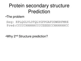
How to evaluate a prediction? The Q3 test: correctly predicted residues number of residues Of course, all methods would be tested on the same proteins.
Calculate propensity of each type of amino acid i using CHOU- FASMAN ALGORITHM Propensities > 1 mean that the residue type I is likely to be found in the Corresponding secondary structure type.
Amino Acid -Helix -Sheet Turn Ala 1.29 0.90 0.78 Cys 1.11 0.74 0.80 Leu 1.30 1.02 0.59 Met 1.47 0.97 0.39 Glu 1.44 0.75 1.00 Gln 1.27 0.80 0.97 His 1.22 1.08 0.69 Lys 1.23 0.77 0.96 Val 0.91 1.49 0.47 Ile 0.97 1.45 0.51 Phe 1.07 1.32 0.58 Tyr 0.72 1.25 1.05 Trp 0.99 1.14 0.75 Thr 0.82 1.21 1.03 Gly 0.56 0.92 1.64 Ser 0.82 0.95 1.33 Asp 1.04 0.72 1.41 Asn 0.90 0.76 1.23 Pro 0.52 0.64 1.91 Arg 0.96 0.99 0.88 Chou-Fasman Rules (Mathews, Van Holde, Ahern) Favors -Helix Favors -Sheet Favors Turns
Chou-Fasman • First widely used procedure • If propensity in a window of six residues (for a helix) is above a certain threshold the helix is chosen as secondary structure. • If propensity in a window of five residues (for a beta strand) is above a certain threshold then beta strand is chosen. • The segment is extended until the average propensity in a 4 residue window falls below a value. • Output-helix, strand or turn.
GOR method • Garnier, Osguthorpe & Robson • Assumes amino acids up to 8 residues on each side influence the ss of the central residue. • Frequency of amino acids at the central position in the window, and at -1, .... -8 and +1,....+8 is determined for a, b and turns (later other or coils) to give three 17 x 20 scoring matrices. • Calculate the score that the central residue is one type of ss and not another. • Correctly predicts ~64%.
I(Sj;R1,R2,…..Rlast) ≃ ∑ I(Sj;Rj+m) m = +8 m = – 8
Artificial Neural Network General structure of ANN : • One input layer. • Some hidden layers. • One output layer.
Architecture Weights Input Layer I K H Output Layer E E E C H V I I Q A E Hidden Layer Window IKEEHVIIQAEFYLNPDQSGEF…..
Secondary Structure Prediction • Application of Multiple sequence alignment • Segment based (+8 to -8 residue) • Input Multiple alignment instead of single seq uence • Application of PSIBLAST • Current methods (combination of) • Segment based • Neural network • Multiple sequence alignment (PSIBLAST) • Combination of Neural Network + Nearest Neighbour Method
PSI - PRED Reliability numbers: • The way the ANN tells us • how much it is sure about • the assignment. • Used by many methods. • Correlates with accuracy.
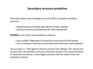
PSIPRED • Uses multiple aligned sequences for prediction. • Uses training set of folds with known structure. • Uses a two-stage neural network to predict structure based on position specific scoring matrices generated by PSI-BLAST (Jones, 1999) • First network converts a window of 15 aa’s into a raw score of h,e (sheet), c (coil) or terminus • Second network filters the first output. For example, an output of hhhhehhhh might be converted to hhhhhhhhh. • Can obtain a Q3 value of 70-78% (may be the highest achievable)
CAFASP3 in the Spotlight of EVAPROTEINS: Structure, Function, and Genetics (2003) 53:548