Download
1 / 45
490 likes | 1.06k Vues
The Smoothed Analysis of Algorithms: Simplex Methods and Beyond. Shang-Hua Teng Boston University/Akamai. Joint work with Daniel Spielman (MIT). Outline. Why. What. Simplex Method. Numerical Analysis. Condition Numbers/Gaussian Elimination. Conjectures and Open Problems.

E N D
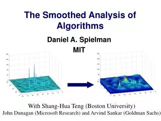
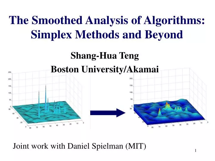
The Smoothed Analysis of Algorithms:Simplex Methods and Beyond Shang-Hua Teng Boston University/Akamai Joint work with Daniel Spielman (MIT)
Outline Why What Simplex Method Numerical Analysis Condition Numbers/Gaussian Elimination Conjectures and Open Problems
Motivation for Smoothed Analysis Wonderful algorithms and heuristics that work well in practice, but whose performance cannot be understood through traditional analyses. worst-case analysis: if good, is wonderful. But, often exponential for these heuristics examines most contrived inputs average-case analysis: a very special class of inputs may be good, but is it meaningful?
Analyses of Algorithms: worst case maxx T(x) average case Er T(r) smoothed complexity
Instance of smoothed framework x is Real n-vector sr is Gaussian random vector, variance s2 measure smoothed complexity as function of n and s
Complexity Landscape run time input space
Complexity Landscape worst case run time input space
average case Complexity Landscape worst case run time input space
Smoothed Complexity Landscape run time input space
Smoothed Complexity Landscape run time smoothed complexity input space
Smoothed Analysis of Algorithms • Interpolate between Worst case and Average Case. • Consider neighborhood of every input instance • If low, have to be unlucky to find bad input instance
Motivating Example: Simplex Method for Linear Programming max zT x s.t. A x £ y • Worst-Case: exponential • Average-Case: polynomial • Widely used in practice
Carbs Protein Fat Iron Cost 1 slice bread 30 5 1.5 10 30¢ 1 cup yogurt 10 9 2.5 0 80¢ 2tsp Peanut Butter 6 8 18 6 20¢ US RDA Minimum 300 50 70 100 The Diet Problem Minimize 30 x1 + 80 x2 + 20 x3 s.t. 30x1 + 10 x2 + 6 x3 300 5x1 + 9x2 + 8x3 50 1.5x1 + 2.5 x2 + 18 x3 70 10x1 + 6 x3 100 x1, x2, x3 0
The Simplex Method opt start
History of Linear Programming • Simplex Method (Dantzig, ‘47) • Exponential Worst-Case (Klee-Minty ‘72) • Avg-Case Analysis (Borgwardt ‘77, Smale ‘82, Haimovich, Adler, Megiddo, Shamir, Karp, Todd) • Ellipsoid Method (Khaciyan, ‘79) • Interior-Point Method (Karmarkar, ‘84) • Randomized Simplex Method (mO(d) ) (Kalai ‘92, Matousek-Sharir-Welzl ‘92)
max zT x s.t. A x £ y max zT x s.t. G is Gaussian Smoothed Analysis of Simplex Method [Spielman-Teng 01] Theorem: For all A, simplex method takes expected time polynomial
Shadow vertex pivot rule start z objective
Theorem:For every plane, the expected size of the shadow of the perturbed tope is poly(m,d,1/s )
Polar Linear Program z max zÎ ConvexHull(a1, a2, ..., am)
Initial Simplex Opt Simplex
[ ] Different Facets < c/N Pr Count pairs in different facets So, expect c Facets
Intuition for Smoothed Analysis of Simplex Method After perturbation, “most” corners have angle bounded away from flat opt start most: some appropriate measure angle: measure by condition number of defining matrix
Condition number at corner Corner is given by Condition number is • sensitivity of x to change in C and b • distance of C to singular
Condition number at corner Corner is given by Condition number is
Connection to Numerical Analysis Measure performance of algorithms in terms of condition number of input Average-case framework of Smale: 1. Bound the running time of an algorithm solving a problem in terms of its condition number. 2. Prove it is unlikely that a random problem instance has large condition number.
Connection to Numerical Analysis Measure performance of algorithms in terms of condition number of input Smoothed Suggestion: 1. Bound the running time of an algorithm solving a problem in terms of its condition number. 2’. Prove it is unlikely that a perturbed problem instance has large condition number.
Edelman ‘88: for standard Gaussian random matrix Condition Number Theorem: for Gaussian random matrix variance centered anywhere [Sankar-Spielman-Teng 02]
Edelman ‘88: for standard Gaussian random matrix Condition Number Theorem: for Gaussian random matrix variance centered anywhere (conjecture) [Sankar-Spielman-Teng 02]
Gaussian Elimination • A = LU • Growth factor: • With partial pivoting, can be 2n • Precision needed (n )bits • For every A,
Condition Number and Iterative LP Solvers Renegar defined condition number for LP maximize subject to • distance of (A, b, c) to ill-posed linear program • related to sensitivity of x to change in (A,b,c) Number of iterations of many LP solvers bounded by function of condition number: Ellipsoid, Perceptron, Interior Point, von Neumann
Smoothed Analysis of Perceptron Algorithm [Blum-Dunagan 01] Theorem: For perceptron algorithm Bound through “wiggle room”, a condition number Note: slightly weaker than a bound on expectation
Compare: worst-case complexity of IPM is iterations, note Smoothed Analysis of Renegar’s Cond Number Theorem: [Dunagan-Spielman-Teng 02] Corollary: smoothed complexity of interior point method is for accuracy e
Perturbations of Structured and Sparse Problems Structured perturbations of structured inputs perturb Zero-preserving perturbations of sparse inputs perturb non-zero entries Or, perturb discrete structure…
Goals of Smoothed Analysis Relax worst-case analysis Maintain mathematical rigor Provide plausible explanation for practical behavior of algorithms Develop a theory closer to practice http://math.mit.edu/~spielman/SmoothedAnalysis
Geometry of should be d1/2 (union bound)
Improving bound on For , Apply to random conjecture Lemma: So
Compare: worst-case complexity of IPM is iterations, note Smoothed Analysis of Renegar’s Cond Number Theorem: [Dunagan-Spielman-Teng 02] Corollary: smoothed complexity of interior point method is for accuracy e conjecture