Download
1 / 38
380 likes | 397 Vues
Software Metrics and Design Principles. What is Design?. Design is the process of creating a plan or blueprint to follow during actual construction Design is a problem-solving activity that is iterative in nature

E N D
What is Design? • Design is the process of creating a plan or blueprint to follow during actual construction • Design is a problem-solving activity that is iterative in nature • In traditional software engineering the outcome of design is the design document or technical specification (if emphasis on notation)
“Wicked Problem” • Software design is a “Wicked Problem” • Design phase can’t be solved in isolation • Designer will likely need to interact with users for requirements, programmers for implementation • No stopping rule • How do we know when the solution is reached? • Solutions are not true or false • Large number of tradeoffs to consider, many acceptable solutions • Wicked problems are a symptom of another problem • Resolving one problem may result in a new problem elsewhere; software is not continuous
Systems-Oriented Approach • The central question: how to decompose a system into parts such that each part has lower complexity than the system as a whole, while the parts together solve the user’s problem? • In addition, the interactions between the components should not be too complicated • Vast number of design methods exist
Design Considerations • “Module” used often – usually refers to a method or class • In the decomposition we are interested in properties that make the system flexible, maintainable, reusable • Information Hiding • System Structure • Complexity • Abstraction • Modularity
Abstraction • Abstraction • Concentrate on the essential features and ignore, abstract from, details that are not relevant at the level we are currently working on • E.g. Sorting Module • Consider inputs, outputs, ignore details of the algorithms until later • Two general types of abstraction • Procedural Abstraction • Data Abstraction
Procedural Abstraction • Fairly traditional notion • Decompose problem into sub-problems, which are each handled in turn, perhaps decomposing further into a hierarchy • Methods may comprise the sub-problems and sub-modules, often in time
Data Abstraction • From primitive to complex to abstract data types • E.g. Integers to Binary Tree to Data Store for Employee Records • Find hierarchy in the data
Modularity • During design the system is decomposed into modules and the relationships among modules are indicated • Two structural design criteria as to the “goodness” of a module • Cohesion : Glue for intra-module components • Coupling : Strength of inter-module connections
Levels of Cohesion • Coincidental • Components grouped in a haphazard way • Logical • Tasks are logically related; e.g. all input routines. Routines do not invoke one another. • Temporal • Initialization routines; components independent but activated about the same time • Procedural • Components that execute in some order • Communicational • Components operate on the same external data • Sequential • Output of one component serves as input to the next component • Functional • All components contribute to one single function of the module • Often transforms data into some output format
Using Program and Data Slices to Measure Program Cohesion • Bieman and Ott introduced a measure of program cohesion using the following concepts from program and data slices: • A data token is any variable or constant in the module • A slice within a module is the collection of all the statements that can affect the value of some specific variable of interest. • A data slice is the collection of all the data tokens in the slice that will affect the value of a specific variable of interest. • Glue tokens are the data tokens in the module that lie in more than one data slice. • Super glue tokens are the data tokens in the module that lie in every data slice of the program Measure Program Cohesion through 2 metrics: - weak functional cohesion = (# of glue tokens) / (total # of data tokens) - strong functional cohesion = (#of super glue tokens) / (total # of data tokens)
Procedure Sum and Product (N : Integer; Var SumN, ProdN : Integer); Var I : Integer Begin SumN : = 0; ProdN : = 1; For I : = 1 to N do begin SumN : = SumN + I ProdN: = ProdN * I End; End;
Data Slice for SumN ( N : Integer; Var SumN, ProdN : Integer); Var I : Integer Begin SumN : = 0; ProdN : = 1; For I : = 1 to N do begin SumN : = SumN + I ProdN: = ProdN * I End; End; Data Slice for SumN = N1·SumN1·I1·SumN2·01·I2·12·N2·SumN3·SumN4·I3
Data Slice for ProdN ( N : Integer; Var SumN, ProdN : Integer); Var I : Integer Begin SumN : = 0; ProdN : = 1; For I : = 1 to N do begin SumN : = SumN + I ProdN: = ProdN * I End; End; Data Slice for ProdN = N1·ProdN1·I1·ProdN2·11·I2·12·N2·ProdN3·ProdN4·I4
Super Glue S1 S2 S3 I I I Super Glue I I I I I I Super Glue I I I Glue I I Glue
Functional Cohesion • Strong functional cohesion (SFC) in this case is the same as WFC SFC = 5/17= 0.204 • If we had computed only SumN or ProdN then • SFC = 17/17= 1
Coupling • Measure of the strength of inter-module connections • High coupling indicates strong dependence between modules • Should study modules as a pair • Change to one module may ripple to the next • Loose coupling indicates independent modules • Generally we desire loose coupling, easier to comprehend and adapt
Types of Coupling • Content • One module directly affects the workings of another • Occurs when a module changes another module’s data • Generally should be avoided • Common • Two modules have shared data, e.g. global variables • External • Modules communicate through an external medium, like a file • Control • One module directs the execution of another by passing control information (e.g. via flags) • Stamp • Complete data structures or objects are passed from one module to another • Data • Only simple data is passed between modules
Modern Coupling • Modern programming languages allow private, protected, public access • Coupling may be modified to indicate levels of visibility, whether coupling is commutative • Simple Interfaces generally desired • Weak coupling and strong cohesion • Communication between programmers simpler • Correctness easier to derive • Less likely that changes will propagate to other modules • Reusability increased • Comprehensibility increased
Cohesion and Coupling Tight High Level Strong Cohesion Coupling Weak Loose Low Level
Dharma (1995) • Data and control flow coupling • di = number of input data parameters • ci = number of input control parameters • do = number of output data parameters • co = number of output control parameters • Global coupling • gd = number of global variables used as data • gc = number of global variables used as control • Environmental coupling • w = number of modules called (fan-out) • r = number of modules calling the module under consideration (fan-in)
Dharma (1995) • Coupling metric (mc) mc = k/M, where k = 1 M = di + a* ci + do + b* co + gd + c* gc + w + r where a=b=c=2 • The more situations encountered, the greater the coupling, and the smaller mc • One problem is parameters and calling counts don’t guarantee the module is linked to the inner workings of other modules
Henry-Kafura (Fan-in and Fan-out) • Henry and Kafura metric measures the inter-modular flow, which includes: • Parameter passing • Global variable access • inputs • outputs • Fan-in : number of inter-modular flow into a program • Fan-out: number of inter-modular flow out of a program Module, P Module’s Complexity, Cp = ( fan-in x fan-out ) 2 for example above: Cp = (3 + 1) 2 = 16
Information Hiding • Each module has a secret that it hides from other modules • Secret might be inner-workings of an algorithm • Secret might be data structures • By hiding the secret, changes do not permeate the module’s boundary, thereby • Decreasing the coupling between that module and its environment • Increasing abstraction • Increasing cohesion (the secret binds the parts of a module) • Design involves a series of decisions. For each such decision, questions are: who needs to know about these decisions? And who can be kept in the dark?
Complexity • Complexity refers to attributes of software that affect the effort needed to construct or change a piece of software • Internal attributes; need not execute the software to determine their values • Many different metrics exist to measure complexity • Two broad classes • Intra-Modular attributes • Inter-Modular attributes
Intra-Modular Complexity • Two types of intra-modular attributes • Size-Based Metrics • E.g. Lines of Code • Obvious objections but still commonly used • Structure-Based Metrics • E.g. complexity of control or data structures
Halstead’s Software Science • Size-based metric • Uses number of operators and operands in a piece of software • n1 is the number of unique operators • n2 is the number of unique operands • N1 is the total number of occurrences of operators • N2 is the total number of occurrences of operands • Halstead derives various entities • Size of Vocabulary: n = n1+n2 • Program Length: N = N1+N2 • Program Volume: V = Nlog2n • Visualized as the number of bits it would take to encode the program being measured
Halstead’s Software Science • Potential Volume: V* = (2+n2)log(2+n2) • V* is the volume for the most compact representation for the algorithm, assuming only two operators: the name of the function and a grouping operator. n2 is minimal number of operands. • Program Level: L = V*/V • Programming Effort: E = V/L • Programming Time in Seconds: T = E/18 • Numbers derived empirically, also based on speed human memory processes sensory input Halstead metrics really only measures the lexical complexity, rather than structural complexity of source code.
Software Science Example • procedure sort(var x:array; n: integer) • var i,j,save:integer; • begin • for i:=2 to n do • for j:=1 to i do • if x[i]<x[j] then • begin save:=x[i]; • x[i]:=x[j]; • x[j]:=save • end • end
Software Science Example Size of vocabulary: 21 Program length: 60 Program volume: 264 Program level: 0.04 Programming effort: 6000 Estimated time: 333 seconds
Structure-Based Complexity • McCabe’s Cyclomatic Complexity • Create a directed graph depicting the control flow of the program • CV = e – n + 2p • CV = Cyclomatic Complexity • e = Edges • n = nodes • p = connected components
Cyclomatic Example For Sorting Code; numbers refer to line numbers 1 2 3 4 5 6 10 7 8 9 11 CV = 13 – 11 + 2*1 = 4 McCabe suggests an upper limit of 10 • T.J. McCabe’s Cyclomatic complexity metric is based on the belief that program quality is related to the complexity of the program control flow.
Shortcomings of Complexity Metrics • Not context-sensitive • Any program with five if-statements has the same cyclomatic complexity • Measure only a few facts; e.g. Halstead’s method doesn’t consider control flow complexity • Others? • Minix: • Of the 277 modules, 34 have a CV > 10 • Highest has 58; handles ASCII escape sequences. A review of the module was deemed “justifiably complex”; attempts to reduce complexity by splitting into modules would increase difficulty to understand and artificially reduce the CV
System Structure – Inter-Module Complexity • The design may consist of modules and their relationships • Can denote this in a graph; nodes are modules and edges are relationships between modules • Types of inter-module relationships: • Module A contains Module B • Module A follows Module B • Module A delivers data to Module B • Module A uses Module B • We are mostly interested in the last one, which manifests itself via a call graph • Possible shapes: • Chaotic • Directed Acyclic Graph (Hierarchy) • Layered Graph (Strict Hierarchy) • Tree
Graph Metrics • Metrics use: • Size of the graph • Depth • Width (maximum number of nodes at some level) • A tree-like call graph is considered the best design • Some metrics measure the deviation from a tree; the tree impurity of the graph • Compute number of edges that must be removed from the graph’s minimum spanning tree • Other metrics • Complexity(M) = fanin(M)*fanout(M) • Fanin/Fanout = local and global data flows
Software Metrics Etiquette • Use common sense and organizational sensitivity when interpreting metrics data. • Provide regular feedback to the individuals and teams who have worked to collect measures and metrics. • Don’t use metrics to appraise individuals • Work with practitioners and teams to set clear goals and metrics that will be used to achieve them. • Never use metrics to threaten individuals or teams. • Metrics data that indicate a problem area should not be considered “negative”. These data are merely an indicator for process improvement. • Don’t obsess on a single metric to the exclusion of other important metrics.