Download
1 / 58
580 likes | 598 Vues
Introduction to Quantum Chemistry Dr. Mazin A Othman. I: Foundations of Quantum Chemistry 1. Classical Chemistry 1.1 Features of classical mechanics. 1.2 Some relevant equations in classical mechanics. 1.3 Example – The 1-Dimensional Harmonic Oscillator

E N D
Introduction to Quantum ChemistryDr. Mazin A Othman I: Foundations of Quantum Chemistry 1.Classical Chemistry 1.1 Features of classical mechanics. 1.2 Some relevant equations in classical mechanics. 1.3Example – The 1-Dimensional Harmonic Oscillator 1.4 Experimental evidence for the breakdown of classical mechanics. 1.5 The Bohr model of the atom. 2. Wave-Particle Duality 2.1Waves behaving as particles. 2.2 Particles behaving as waves. 2.3 The De Broglie Relationship.
3. Wavefunctions 3.1 Definitions. 3.2 Interpretation of the wavefunction.. 3.3 Normalization of the wavefunction. 3.4 Quantization of the wavefunction 3.5 Heisenberg’s Uncertainty Principle. 4. Wave Mechanics 4.1Operators and observables. 4.2 The Schrödinger equation. 4.3 Particle in a 1-dimensional box. 4.4 Further examples.
Learning Objectives • To appreciate the differences between Classical (CM) and Quantum Mechanics (QM). • To know the failures in CM that led to the development of QM. • To know how to interpret the wavefunction and how to normalize it. • To appreciate the origins and implications of quantization and the uncertainty principle. • To understand wave-particle duality and know the relationships between momentum, frequency, wavelength and energy for “particles” and “waves”. • To be able to write down the Schrödinger equation for particles: in a 1-D box; in 1- and 2-electron atoms; in 1- and 2-electron molecules. • To know the origins and allowed values of atomic quantum numbers and how the energies and angular momenta of hydrogen atomic orbitals depend on them. • To be able to sketch the angular and radial nodal properties of atomic orbitals. • To appreciate the origins of sheilding and its effect on the ordering of orbital energies in many-electron atoms.
To use the Aufbau Principle, the Pauli Principle and Hund’s Rule to predict the lowest energy electron configuration for many-electron atoms. • To appreciate how the Born-Oppenheimer approximation can be used to separate electronic and nuclear motion in molecules. • To understand how molecular orbitals (MOs) can be generated as linear combinations of atomic orbitals and the difference between bonding and antibonding orbitals. • To be able to sketch MOs and their corresponding electron densities. • To construct MO diagrams for homonuclear and heteronuclear diatomic molecules. • To predict the electron configurations for diatomic molecules, calculate bond orders and relate these to bond lengths, strengths and vibrational frequencies.
References Fundamentals • P. W. Atkins, J. de Paula, Atkins' Physical Chemistry (7th edn.), OUP, Oxford, 2001. • D. O. Hayward, Quantum Mechanics for Chemists (RSC Tutorial Chemistry Texts 14) Royal Society of Chemistry, 2002. • W. G. Richards and P. R. Scott, Energy Levels in Atoms and Molecules (Oxford Chemistry Primers 26) OUP, Oxford, 1994. More Advanced • P. W. Atkins and R. S. Friedman, Molecular Quantum Mechanics (3rd edn.) OUP, Oxford, 1997. • P. A. Cox, Introduction to Quantum Theory and Atomic Structure (Oxford Chemistry Primers 37) OUP, Oxford, 1996.
1. Classical Mechanics • Do the electrons in atoms and molecules obey Newton’s classical laws of motion? • We shall see that the answer to this question is “No”. • This has led to the development of Quantum Mechanics – we will contrast classical and quantum mechanics.
velocityv position r = (x,y,z) 1.1 Features of Classical Mechanics (CM) 1) CM predicts a precise trajectory for a particle. • The exact position (r)and velocity (v) (and hence the momentump = mv) of a particle (mass = m) can be known simultaneously at each point in time. • Note: position (r),velocity (v) and momentum (p) are vectors, having magnitude and direction v = (vx,vy,vz).
Any type of motion (translation, vibration, rotation) can have any value of energy associated with it – i.e. there is acontinuum of energy states. • Particles and waves are distinguishable phenomena, with different, characteristic properties and behaviour. PropertyBehaviour mass momentum Particles position collisions velocity Waves wavelength diffraction frequency interference
1.2 Revision of Some Relevant Equations in CM Total energy of particle: E= Kinetic Energy (KE) +Potential Energy (PE) E =½mv2+ V E =p2/2m+ V (p = mv) Note: strictly E, T, V (and r, v, p) are all defined at a particular time (t) – E(t) etc.. T-depends on v V-depends on r V depends on the system e.g. positional, electrostatic PE
acceleration • Consider a 1-dimensional system (straight line translational motion of a particle under the influence of a potential acting parallel to the direction of motion): • Define: position r = x velocity v = dx/dt momentum p = mv = m(dx/dt) PE V force F = (dV/dx) • Newton’s 2nd Law of Motion F = ma = m(dv/dt) = m(d2x/dt2) • Therefore, if we know the forces acting on a particle we can solve a differential equation to determine it’s trajectory {x(t),p(t)}.
x = 0 F k m x 1.3 Example – The 1-Dimensional Harmonic Oscillator NB – assuming no friction or other forces act on the particle (except F). • The particle experiences a restoring force (F) proportional to its displacement (x) from its equilibrium position (x=0). • Hooke’s Law F = kx k is the stiffness of the spring (or stretching force constant of the bond if considering molecular vibrations) • Substituting F into Newton’s 2nd Law we get: m(d2x/dt2) = kx a (second order) differential equation k
Solution: position x(t) = Asin(t) of particle frequency = /2 = (of oscillation) Note: frequency depends only on characteristics of the system (m,k) – not the amplitude (A)! x time period = 1/ +A t A
Assuming that the potential energy V = 0 at x = 0, it can be shown that the total energy of the harmonic oscillator is given by: E = ½kA2 • As the amplitude (A) can take any value, this means that the energy (E) can also take any value – i.e. energy is continuous. • At any time (t), the position {x(t)} and velocity {v(t)} can be determined exactly – i.e. the particle trajectory can be specified precisely. • We shall see that these ideas of classical mechanics fail when we go to the atomic regime (where E and m are very small) – then we need to consider Quantum Mechanics. • CM also fails when velocity is very large (as v c), due to relativistic effects.
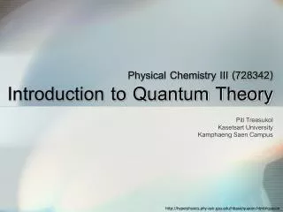
“UV Catastrophe” Classical Mechanics (Rayleigh-Jeans) Energy 2000 K Radiated 1750 K 1250 K 0 2000 4000 6000 1.4 Experimental Evidence for the Breakdown of Classical Mechanics • By the early 20th century, there were a number of experimental results and phenomena that could not be explained by classical mechanics. a) Black Body Radiation (Planck 1900) l /nm
Planck’s Quantum Theory • Planck (1900) proposed that the light energy emitted by the black body is quantized in units of h ( = frequency of light). E = nh (n = 1, 2, 3, …) • High frequency light only emitted if thermal energykT h. • h – a quantum of energy. • Planck’s constanth ~ 6.6261034 Js • If h 0 we regain classical mechanics. • Conclusions: • Energy is quantized (not continuous). • Energy can only change by well defined amounts.
b)Heat Capacities (Einstein, Debye 1905-06) • Heat capacity – relates rise in energy of a material with its rise in temperature: CV = (dU/dT)V • Classical physics CV,m = 3R (for all T). • Experiment CV,m < 3R (CV as T). • At low T, heat capacity of solids determined by vibrations of solid. • Einstein and Debye adopted Planck’s hypothesis. • Conclusion: vibrational energy in solids is quantized: • vibrational frequencies of solids can only have certain values () • vibrational energy can only change by integer multiples of h.
Photoelectrons ejected with kinetic energy: Ek = hn - hn e Metal surface work function = F c) Photoelectric Effect (Einstein 1905) • Ideas of Planck applied to electromagnetic radiation. • No electrons are ejected (regardless of light intensity) unless nexceeds a threshold value characteristic of the metal. • Ek independent of light intensity but linearly dependent on n. • Even if light intensity is low, electrons are ejected if nis above the threshold. (Number of electrons ejected increases with light intensity). • Conclusion: Light consists of discrete packets (quanta) of energy = photons (Lewis, 1922).
d) Atomic and Molecular Spectroscopy • It was found that atoms and molecules absorb and emit light only at specific discrete frequencies spectral lines (not continuously!). • e.g. Hydrogen atom emission spectrum (Balmer 1885) • Empirical fit to spectral lines (Rydberg-Ritz): n1, n2 (> n1) = integers. • Rydberg constant RH = 109,737.3 cm-1 (but can also be expressed in energy or frequency units). n1 = 1 Lyman n1 = 2 Balmer n1 = 3 Paschen n1 = 4 Brackett n1 = 5 Pfund
Revision: Electromagnetic Radiation A – Amplitude l – wavelength n - frequency c = nx l or n= c / l wavenumbern= n / c= 1 / l c (velocity of light in vacuum) = 2.9979 x 10⁸ m s-1.
e n2 E2 E2 n1 h h p+ E1 E1 Absorption Emission 1.5 The Bohr Model of the Atom • The H-atom emission spectrum was rationalized by Bohr (1913): • Energies of H atom are restricted to certain discrete values (i.e. electron is restricted to well-defined circular orbits, labelled by quantum numbern). • Energy (light) absorbed in discrete amounts (quanta = photons), corresponding to differences between these restricted values: E = E2 E1 = h • Conclusion: Spectroscopy provides direct evidence for quantization of energies (electronic, vibrational, rotational etc.) of atoms and molecules.
Limitations of Bohr Model & Rydberg-Ritz Equation • The model only works for hydrogen (and other one electron ions) – ignores e-e repulsion. • Does not explain fine structure of spectral lines. • Note: The Bohr model (assuming circular electron orbits) is fundamentally incorrect.
2. Wave-Particle Duality • Remember: Classically, particles and waves are distinct: • Particles – characterised by position, mass, velocity. • Waves – characterised by wavelength, frequency. • By the 1920s, however, it was becoming apparent that sometimes matter (classically particles) can behave like waves and radiation (classically waves) can behave like particles.
2.1 Waves Behaving as Particles • The Photoelectric Effect Electromagnetic radiation of frequency can be thought of as being made up of particles (photons), each with energy E = h . This is the basis of Photoelectron Spectroscopy (PES). • Spectroscopy Discrete spectral lines of atoms and molecules correspond to the absorption or emission of a photon of energy h , causing the atom/molecule to change between energy levels: E = h . Many different types of spectroscopy are possible.
Intensity s i i s • The Compton Effect (1923) • Experiment: A monochromatic beam of X-rays (i) = incident on a graphite block. • Observation: Some of the X-rays passing through the block are found to have longer wavelengths (s).
p=h/s s i e p=mev • Explanation: The scattered X-rays undergo elastic collisions with electrons in the graphite. • Momentum (and energy) transferred from X-rays to electrons. • Conclusion: Light (electromagnetic radiation) possesses momentum. • Momentum of photonp = h/ • Energy of photonE = h = hc/ • Applying the laws of conservation of energy and momentum we get:
2.2 Particles Behaving as Waves Electron Diffraction (Davisson and Germer, 1925) Davisson and Germer showed that a beam of electrons could be diffracted from the surface of a nickel crystal. Diffraction is a wave property – arises due to interference between scattered waves. This forms the basis of electron diffraction – an analytical technique for determining the structures of molecules, solids and surfaces (e.g. LEED). NB: Other “particles” (e.g. neutrons, protons, He atoms) can also be diffracted by crystals.
2.3 The De Broglie Relationship (1924) • In 1924 (i.e. one year before Davisson and Germer’s experiment), De Broglie predicted that all matter has wave-like properties. • A particle, of mass m, travelling at velocity v, has linear momentum p = mv. • By analogy with photons, the associated wavelength of the particle () is given by:
3. Wavefunctions • A particle trajectory is a classical concept. • In Quantum Mechanics, a “particle” (e.g. an electron) does not follow a definite trajectory {r(t),p(t)}, but rather it is best described as being distributed through space like a wave. 3.1 Definitions • Wavefunction () – a wave representing the spatial distribution of a “particle”. • e.g. electrons in an atom are described by a wavefunction centred on the nucleus. • is a function of the coordinates defining the position of the classical particle: • 1-D (x) • 3-D (x,y,z) =(r) =(r,,) (e.g. atoms) • may be time dependent – e.g. (x,y,z,t)
The Importance of • completely defines the system (e.g. electron in an atom or molecule). • If is known, we can determine any observable property (e.g. energy, vibrational frequencies, …) of the system. • QM provides the tools to determine computationally, to interpret and to use to determine properties of the system.
3.2 Interpretation of the Wavefunction • In QM, a “particle” is distributed in space like a wave. • We cannot define a position for the particle. • Instead we define a probability of finding the particle at any point in space. The Born Interpretation (1926) “The square of the wavefunction at any point in space is proportional to the probability of finding the particle at that point.” • Note: the wavefunction () itself has no physical meaning.
probability density 1-D System • If the wavefunction at point x is (x), the probability of finding the particle in the infinitesimally small region (dx) between x and x+dx is: P(x) (x)2dx • (x)– the magnitude of at point x. Why write 2instead of 2? • Becausemay be imaginary or complex 2would be negative or complex. • BUT: probability must be real and positive (0 P 1). • For the general case, where is complex (= a + ib) then: 2=*where *is the complex conjugate of. (*= a – ib) (NB )
3-D System • If the wavefunction at r = (x,y,z) is (r), the probability of finding the particle in the infinitesimal volume element d (= dxdydz) is: P(r) (r)2d • If (r) is the wavefunction describing the spatial distribution of an electron in an atom or molecule, then: (r)2 = (r) – the electron density at point r
3.3 Normalization of the Wavefunction • As mentioned above, probability: P(r) (r)2 d • What is the proportionality constant? • If is such that the sum of (r)2at all points in space = 1, then: P(x) = (x)2 dx 1-D P(r) = (r)2 d 3-D • As summing over an infinite number of infinitesimal steps = integration, this means: • i.e. the probability that the particle is somewhere in space = 1. • In this case, is said to be a normalized wavefunction.
How to Normalize the Wavefunction • If is not normalized, then: • A corresponding normalized wavefunction (Norm) can be defined: such that: • The factor (1/A) is known as the normalization constant (sometimes represented by N).
3.4 Quantization of the Wavefunction The Born interpretation of places restrictions on the form of the wavefunction: (a)must be continuous (no breaks); (b) The gradient of (d/dx) must be continuous (no kinks); (c)must have a single value at any point in space; (d)must be finite everywhere; (e)cannot be zero everywhere. • Other restrictions (boundary conditions) depend on the exact system. • These restrictions on mean that only certain wavefunctions and only • certain energies of the system are allowed. • Quantization ofQuantization ofE
3.5 Heisenberg’s Uncertainty Principle “It is impossible to specify simultaneously, with precision, both the momentum and the position of a particle*” (*if it is described by Quantum Mechanics) Heisenberg (1927) Dpx.Dx h / 4p (or /2, where = h/2p). Dx– uncertainty in position Dpx– uncertainty in momentum (in the x-direction) • If we know the position (x) exactly, we know nothing about momentum (px). • If we know the momentum (px) exactly, we know nothing about position (x). • i.e. there is no concept of a particle trajectory {x(t),px(t)} in QM (which applies to small particles). • NB – for macroscopic objects, Dx and Dpx can be very small when compared with x and px so one can define a trajectory. • Much of classical mechanics can be understood in the limit h 0.
2 ~ 1 How to Understand the Uncertainty Principle • To localize a wavefunction () in space (i.e. to specify the particle’s position accurately, small Dx) many waves of different wavelengths () must be superimposed largeDpx(p = h/). • The Uncertainty Principle imposes a fundamental (not experimental) limitation on how precisely we can know (or determine) various observables.
Note – to determine a particle’s position accurately requires use of short radiation (high momentum) radiation. Photons colliding with the particle causes a change of momentum (Compton effect) uncertainty in p. The observer perturbs the system. • Zero-Point Energy (vibrational energy Evib 0, even at T = 0 K) is also a consequence of the Uncertainty Principle: • If vibration ceases at T = 0, then position and momentum both = 0 (violating the UP). • Note: There is no restriction on the precision in simultaneously knowing/measuring the position along a given direction (x) and the momentum along another, perpendicular direction (z): • Dpz.Dx= 0
Similar uncertainty relationships apply to other pairs of observables. • e.g. the energy (E) and lifetime () of a state: DE.D (a) This leads to “lifetime broadening” of spectral lines: • Short-lived excited states ( well defined, small D) possess large uncertainty in the energy (largeDE) of the state. • Broad peaks in the spectrum. • Shorter laser pulses (e.g. femtosecond, attosecond lasers) have broader energy (therefore wavelength) band widths. (1 fs = 1015 s, 1 as = 1018 s)
4. Wave Mechanics • Recall – the wavefunction () contains all the information we need to know about any particular system. • How do we determine and use it to deduce properties of the system? 4.1 Operators and Observables • If is the wavefunction representing a system, we can write: where Q – “observable” property of system (e.g. energy, momentum, dipole moment …) – operator corresponding to observable Q.
function multiplied by a number Q (eigenvalue) operator Q acting on function (eigenfunction) • This is an eigenvalue equation and can be rewritten as: (Note: can’t be cancelled). Examples:d/dx(eax) = a eax d2/dx2 (sin ax) = a2sin ax
To find and calculate the properties (observables) of a system: 1. Construct relevant operator 2. Set up equation 3. Solve equation allowed values of and Q. Quantum Mechanical Position and Momentum Operators 1. Operator for position in the x-direction is just multiplication by x 2.Operator for linear momentum in the x-direction: (solve first order differential equation , px).
partial derivatives operate on (x,y,z) Constructing Kinetic and Potential Energy QM Operators 1. Write down classical expression in terms of position and momentum. 2. Introduce QM operators for position and momentum. Examples 1. Kinetic Energy Operator in 1-D CMQM 2. KE Operator in 3-D CMQM 3. Potential Energy Operator (a function of position) PE operator corresponds to multiplication by V(x), V(x,y,z) etc. “del-squared”
4.2 The Schrödinger Equation (1926) • The central equation in Quantum Mechanics. • Observable = total energy of system. Schrödinger Equation Hamiltonian Operator ETotal Energy where and E = T + V. • SE can be set up for any physical system. • The form of depends on the system. • Solve SE and corresponding E.
Examples 1.Particle Moving in 1-D(x) • The form of V(x) depends on the physical situation: • Free particleV(x) = 0 for all x. • Harmonic oscillatorV(x) = ½kx2 2.Particle Moving in 3-D(x,y,z) • SE or Note: The SE is a second order differential equation
PE (V) 0 L 0 x 4.3 Particle in a I-D Box System • Particle of mass m in 1-D box of length L. • Position x = 0L. • Particle cannot escape from box as PE V(x)= for x = 0, L (walls). • PE inside box: V(x)= 0 for 0< x < L. 1-D Schrödinger Eqn. (V = 0 inside box).
This is a second order differential equation – with general solutions of the form: = A sin kx+ B cos kx • SE (i.e. E depends on k).
Restrictions on • In principle Schrödinger Eqn. has an infinite number of solutions. • So far we have general solutions: • any value of {A, B, k} any value of {,E}. • BUT – due to the Born interpretation of , only certain values of are physically acceptable: • outside box (x<0, x>L) V = impossible for particle to be outside the box 2= 0 = 0 outside box. • must be a continuous function Boundary Conditions = 0 at x = 0 = 0 at x = L.
0 1 A=0? (or = 0 for all x) sin kL = 0 ? Effect of Boundary Conditions • x = 0 = A sin kx+ B cos kx =B = 0 B = 0 = A sin kxfor all x • x = L= A sin kL =0 sin kL = 0 kL = n n = 1, 2, 3, … (n 0, or = 0 for all x)
Allowed Wavefunctions and Energies • k is restricted to a discrete set of values: k = n/L • Allowed wavefunctions:n = A sin(nx/L) • Normalization: A = (2/L) • Allowed energies: