Download
1 / 26
260 likes | 264 Vues
Total Solar Irradiance: What have we learned from the last three Solar Cycles. Claus Fröhlich CH 7265 Davos Wolfgang. Outline. Total solar irradiance variability: Observations Discussion of the three composites Does the low TSI during recent minimum point to a long-term trend

E N D
Total Solar Irradiance: What have we learned from the last three Solar Cycles Claus Fröhlich CH 7265 Davos Wolfgang Colloquium at KIS, 12.May 2011
Outline • Total solar irradiance variability: Observations • Discussion of the three composites • Does the low TSI during recent minimum point to a long-term trend • Correlation with open field of the Sun • Total solar irradiance variability: Proxy model • TSI modeling by sunspots, faculae and network together with a trend as 4th component • How much of a trend is in UV and EUV irradiance? • Reconstruction of TSI back 1915 • PSI back to 1874 with RGO data • Construction of a MgII index from Mt Willson CaK observations • Reconstruction of the open field from aa index Colloquium at KIS, 12.May 2011
TSI Database 1978 to present Colloquium at KIS, 12.May 2011
TSI Database 1978 to present Only the PMOD composite corrects the HF radiometer for degradation and other changes over the whole period of its operation. This automatically accounts for the changes during the ACRIM gap. After ACRIM gap the PMOD and ACRIM composite agree pretty well. The IRMB composite is based on DIARAD only and the exponential correction for non-exposure dependent changes is confirmed by results from SOVIM. Colloquium at KIS, 12.May 2011
TSI Database 1978 to present An important issue is how real is the low TSI during the recent minimum: ACRIM shows a very similar behaviour during cycle 23 and confirms the low value.There may be some problems with the cycle amplitude of VIRGO. A thorough re-analysis is under way. Colloquium at KIS, 12.May 2011
Estimation of the Uncertainty of the PMOD Composite over a solar cycle -0.051±0.100 0.000±0.01 -0.110±0.10 -0.323±0.16 Note the low recent minimum, being 25% lower relative to the cycle amplitude. The values and uncertainties of the minimum values are given in Wm-2, relative to the minimum between cycles 21 and 22 (for details see Fröhlich, 2009, A&A, 501, L27). Colloquium at KIS, 12.May 2011
How can we explain the low minimum, is it a trend? Colloquium at KIS, 12.May 2011
Indeed is may be part of a trend Colloquium at KIS, 12.May 2011
Possible explanations of the TSI trend The trend could be due to a change of the temperature of the Sun. For explaining the change of TSI between the last two minima we need a 0.25K cooler Sun. It is obvious that such a small change would change Ly- very little; according to Planck’s law by about 1% which is negligible compared to a cycle amplitude of 60%. Another possibility is the contrast of faculae and network at the photosphere which increases with decreasing magnetic field which makes TSI lower at low cycle minima. Colloquium at KIS, 12.May 2011
Proxy Model: from 3 to 4 components Panel A shows CaII K image of the sun as illustration of the influence of active regions (a), faculae (b) and network (c). Panel B is an H image of part of the sun, showing sunspots, faculae and network. All these are effects of surface magnetic fields and we will see, that they cannot explain the trend, so we need to include it as a 4th component. Colloquium at KIS, 12.May 2011
Proxy Model: from 3 to 4 components Sunspots can be modeled from their area and position on the disk by using an appropriate contrast. The result is the photometric sunspot index (PSI), which is given in ppm of TSI and is used as one component of the proxy model. The butterfly diagram of PSI shows clearly the difference between cycle 23 and the previous ones. The vertical black lines show the time of the minima, which are defined at the first appearance of an important group of the new cycle (high latitude and opposite polarity). Colloquium at KIS, 12.May 2011
A new algorithm for the determination of PSI From these corrected areas PSI is calculated region by region. The areas from all observatories are fitted to a polynomial of degree 1-3 depending on the number of days covered by the region. From these fits the mean area for each day within the region is determined together with the corresponding position on the disk. Colloquium at KIS, 12.May 2011
What about the contrast of sunspots? Colloquium at KIS, 12.May 2011
The influence of faculae and network Colloquium at KIS, 12.May 2011
Calibration against TSI over 3 solar cycles -5.7% Ratio lt/st: 1.61 Trend from direct correlation: 0.35 ± 0.14 Wm-2/nT Colloquium at KIS, 12.May 2011
How is the UV/EUV behaviour? Comparing the ascending part of both with the model one could argue that the positive BR slope of SEM and the negative one of Ly- are due to some instrumental trends. Thus, the slope for both could be zero – certainly not 0.322 Wm-2nT-1 as for TSI. Colloquium at KIS, 12.May 2011
Conclusions for TSI over the last 3 Cycle • The PMOD composite is a reliable representation of TSI. The absolute value is still controversial. • The 4-component model for TSI with PSI, a short and long-term MgII index and a trend from BR can explain 84% of the variance. As PSI and MgII alone cannot explain the trend, it must have another origin. • A global temperature change of the Sun between the last two minima of only about 0.25 K is needed to explain the trend. However, the increasing contrast of faculae and network with decreasing magnetic field could be a alternative explanation. • Most of the short-term variation (days to solar-cycle timescales) – if not all - of total and spectral solar irradiance are due to manifestations of surface magnetism. • The long-term trend observed in TSI is directly related to the strength of the activity and thus can be reconstructed accordingly. • With these results TSI can be reconstructed back to 1915 from (a) PSI deduced from the Royal Greenwich Observatory, (b) CaK index from the Mt.Wilson observations and (c) BR from aa index. Colloquium at KIS, 12.May 2011
Results from the 4-Component Model for the Period 1975-2010 can be used Colloquium at KIS, 12.May 2011
What is available for the last century to reconstruct TSI with a 4-component Model Colloquium at KIS, 12.May 2011
MgII index back to 1915 from CaK Observations Colloquium at KIS, 12.May 2011
PSI back to 1874 from RGO and SOON Data Colloquium at KIS, 12.May 2011
Reconstruction of BR since 1880 Colloquium at KIS, 12.May 2011
4-Component Model 1915-20010 Colloquium at KIS, 12.May 2011
The calibration of the 4-component model during 1975-2009 can now be used Colloquium at KIS, 12.May 2011
Comparison of Model and Observed Colloquium at KIS, 12.May 2011
Conclusions on the reconstruction • For the 4-component model back to 1915 the following components have been successfully used: • PSI from sunspot data from RGO and SOON • Open Field BR from reconstructions by the aa index • Decomposed MgII index from CaK observations at Mt.Wilson • For the long-term dependence of TSI we use the correlation with BR. This does not apply to the UV radiation, which means that there is essentially no long-term trend for UV and EUV irradiance – only changes of the amplitude. • The reconstructed TSI is at about the same level during the minimum in 1924/25 as in 2008/09 • The change of TSI from the highest minimum in 1985/86 to the lowest minimum in 1924 is 0.340 Wm-2 or 250 ppm. This presentation can be found on: ftp://ftp.pmodwrc.ch/pub/Claus/KIS%20Colloquium/KIS_Coll_2011.ppt Colloquium at KIS, 12.May 2011