Download
1 / 23
240 likes | 462 Vues
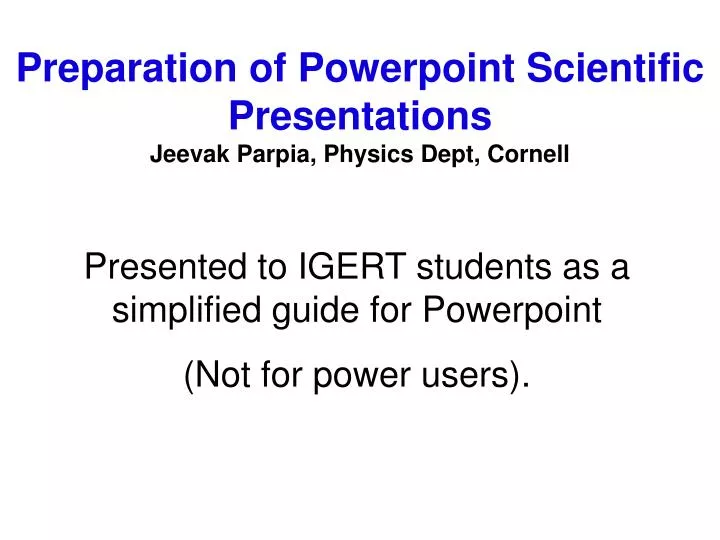
Preparation of Powerpoint Scientific Presentations Jeevak Parpia, Physics Dept, Cornell. Presented to IGERT students as a simplified guide for Powerpoint (Not for power users). The Basics.

E N D
Preparation of Powerpoint Scientific Presentations Jeevak Parpia, Physics Dept, Cornell Presented to IGERT students as a simplified guide for Powerpoint (Not for power users).
The Basics To set your font (open Format, Select Fonts, Then Arial, then check box for default for new objects). Select a size. This 24 pt. The heading is 40 pt (bold). Set line spacing. I have 1 line and 0.3 line between new paragraphs. That improves readability. Don’t use ALL CAPS. Plan on a uniform pattern through the talk, ie a main heading that outlines the point of the slide, and text/graphical information. You can save yourself a bunch of time by making one slide, then duplicating it and replacing information in there. Now lets try animations: From the Slide Show Menu select Custom Animations, and a window opens to your right. You should highlight the previous text, then from the “Animations menu” Go to “Add Effect”, select Emphasis, then “Transparency”. This is 75% Then 50% Try it.
Data from Origin – or Excel (Yes its possible) Squish your text box over to one side. Paste in the graph (which is nasty. Notice that when I click on the graph, it opens Origin.
Data from Origin – or Excel (Yes its possible) Squish your text box over to one side. Paste in the graph (which is nasty. Notice that when I click on the graph, it opens Origin. Whats wrong with it? Axes, labels are dreadful. 36 pt (and shrunken). Hard to read. Do we need that label on there? Or does it belong in text? Fix labels
Data from Origin – or Excel (Yes its possible) I now save the graph from Origin by selecting Export, and then png format, store in the same folder as presentation for easy access. Label in some sensible way. Next I have arranged it so that I can place a rectangle over the inset so I can highlight data should I need to. This eliminates clutter. You could put text here too. Quality factor vs Laser power
Matching Networks and N/MEMSDarren Southworth, Jeevak Parpia & Keith SchwabDept of Physics, Cornell University • The Problem: Hard to get signal into and out of M/NEMS. (Nano/Micro Electro-Mechanical Systems) • Inhibits wider usage of N/MEMS in applications. • We present a simple solution.
Cg=10aF Matching Network 1 Load ZL Zo Γ Caveat: All effects demonstrated at temperatures below 1K. Limits applicability! Matching Networks & M/NEMSDarren Southworth, Jeevak Parpia, Keith SchwabCornell University Impedance Matching Networks • Coupling capacitance to NEMS is v small: 1-10 aF. Even at 1GHz, impedance is 16MΩ! Huge mismatch! • Reflected signal, Γis ~ 1 • Insertion of matching network ensures maximum power delivered. • Treat resonator as RmLmCm , Rm depends crucially on Q! When on resonance, Rm ≈ 0, and reflectance changes.
LT Cg Network Analyzer CT FC3: Summary of Matching Networks -3 Electrically Isolating Trench Dome Resonator Wire Bond Rendition of 1st generation MEMS integrated to matching network 50 µm Rm = 2-8 kΩ Cg = 200 fF Stressed Polysilicon Single Dome Structure Insulating Oxide Silicon Substrate
Optical and Electronic Drive and Readout of MEMS Dome Oscillators Actuation/detection with laser 10µm Resonance at 12.4 MHz with a quality factor around 1000 All electric drive/detection FC3: Summary of Matching Networks -4 All electric drive and detection
Conclusion ● Demonstrated all electrical readout of resonator with matching network. ● Single Coaxial line needed for Actuation/Readout Future Work: ● Optimize matching network for better S/N ● Put network on-chip to gain size advantage ● Explore additional feedback selectively narrow resonance. All electric drive and detection Funded by DARPA, NSF via IGERT, CNF
Harnessing Active Resonant MEMS (HARMs) Jeevak Parpia June 28, 2007 Physics Department, Cornell University
Center Mission Optimize CMOS-integrated, chemically functionalized-surface M/NEMS for sensing. Fundamental Challenges (FC): FC1: Rarified gas dynamics FC2: Surface Chemistry FC3: I/O from NEMS FC4: Integration of NEMS to CMOS
Slide Master All new slides have this format. Consider developing a “Slide Master” for your group Advantages: ●Share slides seamlessly ●Bottom Bar can update group results ●Highlight Funding agencies Disadvantages ●Can be trite ●Occupies real estate ●Discourages individuality
Resources ● Help in toolbar: There are many hours of time savings here. Find useful symbols on the web (if you don’t enjoy drudgery) e.g. for electrical components: ● http://www.wpclipart.com/signs_symbol/electrical/ Or many others at ● http://www.wpclipart.com/downloads.html
20 µm Images for Reports in Word (also useful for ppt) ● Establish width of Figure. 2.5 inch is USUALLY fine. ● Crop unwanted (illegible) bits out e.g. SEM info. ● Show scale bar. You will likely have to regenerate this. ● Compress images to eliminate unwanted bits, and save space. ● Group everything together (from Draw menu). ● Change axes, scales, proportions of excel plot, print to pdf, crop, save as .png. Import & group.
(a) (b) 20 µm (c) Fig 1. (a) Matching network on PC board, mated to DIP chip containing dome resonator (b). Vacuum line (a) exiting to right allows controlled atmosphere, co-ax to left bottom enables signal I/O. (c) resonance obtained with set up. Images for Reports in Word ● Establish width of Figure. 2.5 inch is USUALLY fine. ● Crop unwanted (illegible) bits out e.g. SEM info. ● Show scale bar. You will likely have to regenerate this. ● Compress images to eliminate unwanted bits, and save space. ● Group everything together (from Draw menu). ● Change axes, scales, proportions of excel plot, print to pdf, crop, save as .png. Import & group.
Structure for Posters in pp • Title up top, Authors/Institutions next, poster number usually mandatory. • Introduce directionality – guide reader through poster. Use titles for boxes. • Use colors to segregate portions of text & link ideas together. • I find transporting a poster tedious, consider cutting it for transport ie be sure to include lines where it might be cut. • Put main ideas at eye level (hard to know where that will be).
Great graphics Clear layout Nice features
Scaling Results for Superfluid 3He in 98% open Aerogel 4P4 CONCLUSIONS The close parallels between the observed scaling of Ω2Baand s/ of dirty superfluid 3He is striking evidence that the strength of the superfluid pairing is significantly modified from the bulk behavior. The onset of superfluidity occurs at a nearly pressure independent but sample dependent length scale. Whether this can be related to the observed onset of superfluidity at a particular (presumably sample dependent) value of Ω2B is yet to be explored theoretically. Further, the observation of a very similar power law for the development of the superfluid density and the square of the Leggett frequency is also tantalizing, and it is remarkable that more than ten years after the first observation of dirty superfluidity the power law behavior, and collapse of these data onto nearly universal plots against (Tca-T) have not yet been understood theoretically. It is likely that further understanding will require the development of a relationship between the structure of aerogel to the experimental observations. EXPERIMENTAL RESULTS Fig 1: The square of the Leggett frequency ΩB2observed simultaneously in a bulk sample (solid lines) and in 98.2 aerogel. The suppression of the onset of the superfluid transition, suppression of ΩB and additional curvature of the data in the aerogel are notable. See scaling result in Fig 4 alongside. Fig. 2: The superfluid fraction in bulk (solid lines) and in dirty 3He (3He in 98% aerogel – dashed lines) plotted against the temperature. The suppressed Tc and s/ are evident. The fact that the shapes of these “dirty superfluid densities” replicates when plotted vs Tca-T is borne out by examination of the scaling plot in Fig. 5 alongside. Data from Ref. 1. The upward curvature of the dirty superfluid data is unlikely to be only due to sample inhomogeneities5. Fig. 3:The superfluid transition temperatures for various cells, along with the bulk transition temperatures. A simple relationship to estimate the onset of superfluidity (see accompanying Fig. 6 alongside) yields the dashed lines that closely replicate the transition temperatures. Data from Cell A1, Cell B6, Cell C7, and Moscow3. J.M. Parpiaa, A.D. Feffermana, J.V. Portoa,b, V.V. Dmitrievc, L.V. Levitinc,d, & D.E. Zmeevc. aDepartment of Physics, Cornell University, Ithaca, NY, 14853, USA, bCurrent address: NIST Gaithersburg, MD 20899, USA cKapitza Institute for Physical Problems, Moscow 119334, Russia dCurrent address: Department of Physics, Royal Holloway University of London, Egham, TW20 OEX, UK INTRODUCTION SCALING RESULTS More than a decade ago, experiments1,2 revealed that the addition of silica aerogel alters the properties of superfluid 3He. The most obvious manifestation of these modifications is the suppression of the transition temperature and the reduction of the superfluid fraction, rs/r and its NMR analog, the Leggett frequency ΩB.3 We discuss the observation of specific scaling relations of Tc, rs/r, WBa. Fig 4. The Leggett frequency squared (ΩBa/2π)2observed for 3He-B in 98.2 aerogel plotted against (ΩB/2π)2 simultaneously observed in a bulk 3He-B sample (Ph. D. thesis, Zmeev, Kapitza Inst.). All measured pressures show the onset of superfluidity (characterized by the frequency shift onset), at the same value of ΩB. The Leggett frequency in the B-like phase was measured using the frequency shift for the textural defect3, while the data for bulk 3He were obtained in an additional bulk cell filled with a set of equally spaced plates to orient the texture of the order parameter (see Ref. 4). Fig. 5 The superfluid density rs/r and Leggett frequency squared in the B-like phase of 3He in aerogel, (ΩBa/2π)2, plotted against the temperature below the onset of the superfluid transition Tca-T in mK. For clarity we show only two pressures for rs/r, and three pressures for (ΩBa/2π)2. The near collapse of these is remarkable, as is the similarity of the power law behavior. We find the exponents for the temperature to be 1.38 for the NMR, 1.33 for the low pressure and 1.45 for the high pressure s/. The difference in the superfluid density exponent is likely due to changes when the sample was warmed up between runs. Fig. 6 The reduced transition temperature, √(1-Tca/Tc) at a variety of pressures for various 98% open aerogel samples measured in our laboratories, against the zero temperature coherence length, ξ0(P). The transition temperature observed in 98% open aerogel occurs at a sample dependent (pressure independent) length X = ξ0/ √(1-Tca/Tc). The lines through the data correspond to slopes of 0.0155 nm-1 (X=65 nm) & 0.0225 nm-1 X=44 nm. This simple relation does not work for samples of higher porosity. A similar relation is seen in the so called “slab model”8. REFERENCES & ACKNOWLEDGEMENTS 1. J.V. Porto and J.M. Parpia, Phys. Rev. Lett.74, 4667, (1995) 5. R. Hanninen and E.V. Thuneberg, Phys. Rev. B67, 214507, (2003) 2. D.T. Sprague, T.M. Haard, J.B. Kycia, M.R. Rand, Y. Lee, P.J. Hamot and W.P. Halperin, Phys. Rev. Lett.75, 661, (1995) 6. A. Golov, J.V. Porto and J. M. Parpia, Phys. Rev. Lett. 80, 4486 (1998) 3. V.V. Dmitriev, N. Mulders, V.V. Zavjalov, D. E.Zmeev, AIP Conference Proceedings, 850 229 (2006) 7. K. Matsumoto, J.V. Porto, L. Pollack, E.N. Smith, T.L. Ho and J. M. Parpia, Phys. Rev. Lett. 79, 253 (1997) 4. A.I. Ahonen, M. Krusius and M.A. Paalanen, J. of Low. Temp. Phys., 25, 421 (1976) 8. E.V. Thuneberg, S.K. Yip, M. Fogelstrom, and J.A. Sauls, Phys. Rev. Lett. 80, 2861 (1998) Supported by the N.S.F. under DMR-0457533, the CRDF under RUP1-2632-MO-04, NATO under SA(PST.CLG.979379)6993/FP the Russian Foundation for Basic Research under 06-02-17185, & the Ministry of Science and Education of Russia under NSh-9725.2006.2
Resources for Posters • http://cf.ccmr.cornell.edu/posters.html • http://cf.ccmr.cornell.edu/ScientificPosters.pdf • Posters are expensive to generate. CNF does them for free (they ask you to Minimize large colored areas to conserve ink, so colored backgrounds a no-no for them). • Colors often dont transfer, sometimes pdfs also fail, and there can be back ups. Bottom line -- work ahead.
Poster specs Maximum poster width is 60 inches. Most poster boards are not that wide. Poster can be generated sideways. Check and print (scaled to size) on a color laser printer. Proof prints can also be useful as giveaway flyers to plug your work. Make your –email prominent or print full scale on back.
Acknowledgements • Darren Southworth, Andrew Fefferman, Maxim Zalalutdinov, Keith Schwab (data, images) • Melissa Hines: critique, images