Download
1 / 66
680 likes | 944 Vues
Luminosity measurement at LHC. Coseners Forum 12 th -13 th April 2007 Per Grafstrom CERN. Luminosity measurements-why?. Cross sections for “Standard “ processes t-tbar production W/Z production ……. Theoretically known to better than 10% ……will improve in the future

E N D
Luminosity measurement at LHC Coseners Forum 12th-13th April 2007 Per Grafstrom CERN
Luminosity measurements-why? • Cross sections for “Standard “ processes • t-tbar production • W/Z production • ……. Theoretically known to better than 10% ……will improve in the future • New physics manifesting in deviation of x BR relative the Standard Model predictions • Important precision measurements • Higgs production x BR • tan measurement for MSSM Higgs • …….
Relative precision on the measurement of HBR for various channels, as function of mH, at Ldt = 300 fb–1. The dominant uncertainty is from Luminosity: 10% (open symbols), 5% (solid symbols). (ATLAS-TDR-15, May 1999) Luminosity Measurement (cont.) Examples Higgs coupling tan measurement Systematic error dominated by luminosity (ATLAS Physics TDR )
Absolute vs relative measurement • Strategy: 1. Measure the absolute luminosity with a precise method at optimal conditions 2. Calibrate luminosity monitor with this measurement, which can then be used at different conditions • Luminosity Monitoring i.e. relative measurements: • Using suitable observables in existing detectors • Use dedicated luminosity monitors either provided by the experiments or by the machine Today we will mainly discuss methods for Absolute Luminosity Measuremet
Absolute Luminosity Measurements Goal: Measure L with ≲ 3% accuracy (long term goal) How? Three major approaches • LHC Machine parameters • Rates of well-calculable processes:e.g. QED (like LEP), EW and QCD • Elastic scattering • Optical theorem: forward elastic rate + total inelastic rate: • Luminosity from Coulomb Scattering • Hybrids • Use totmeasured by others • Combine machine luminosity with optical theorem We better pursue all options
Outline • Methods for Absolute Measurement of Luminosity • Use Processes with known cross sections • Use Machine Parameters • Use Elastic scattering
Muon pairs Two photon production of muon pairs-QED p Pure QED Theoretically well understood No strong interaction involving the muons Proton-proton re-scattering can be controlled Cross section known to better than 1 % p
Muon pairs Two photon production of muon pairs Pt 3 GeV to reach the muon chambers Pt6 GeV to maintain trigger efficiency and reasonable rates Centrally produced 2.5 Pt() 10-50 MeV Close to back to back in (background suppression) m- f m+
Muon pairs Backgrounds • Strong interaction of a single proton • Strong interaction between colliding proton • Di-muons from Drell-Yan production • Muons from hadron decay
Muon pairs Event selection-two kind of cuts • Kinematic cuts Pt of muons are equal within 2.5 σ of the measurement uncertainty • Good Vertex fit and no other charged track Suppress Drell-Yan background and hadron decays Suppresses efficiently proton excitations and proton-proton re-scattering
Muon pairs What are the difficulties ? • The rate The kinematical constraints σ 1 pb A typical 1033/cm2/sec year 6 fb -1 and 150 fills 40 events fill Luminosity MONITORING excluded What about LUMINOSITY calibration? 1 % statistical error more than a year of running • Efficiencies Both trigger efficiency and detector efficiency must be known very precisely. Non trivial. • Pile-up Running at 1034/cm2/sec “vertex cut” and “no other charged track cut” will eliminate many good events • CDF result First exclusive two-photon observed in e+e-. …. but…. 16 events for 530 pb-1 for a σ of 1.7 pb overall efficiency 1.6 % Summary– Muon Pairs Cross sections well known and thus a potentially precise method. However it seems that statistics will always be a problem.
W and Z W and Z counting
W and Z W and Z counting • Constantly increasing precision of QCD calculations makes counting of leptonic decays of W and Z bosons a possible way of measuring luminosity. In addition there is a very clean experimental signature through the leptonic decay channel. • Use W in this discussion . (W) x BR(W l) has more favourable rate. The rate is 10 x (Z) x BR(Z ll ). The Basic formula L = (N - BG)/ ( x AW x th) Lis the integrated luminosity N is the number of W candidates BG is the number of back ground events is the efficiency for detecting W decay products AW is the acceptance th is the theoretical inclusive cross section
Pseudorapidity 2.4 (no bias at edge) Pt > 25 GeV (efficient electron ident) Missing Et > 25 GeV No jets with Pt > 30 GeV (QCD background) QCD background and heavy quarks Z e+e- where the second lepton is not identified Z +- where one decay in the electron channel ttbar background W l ; decaying in the electron channel W and Z How to select events and eliminate background(N-BG)
W and Z Uncertainties on th • th is the convolution of the Parton Distribution Functions (PDF) and of the partonic cross section • The uncertainty of the partonic cross section is available to NNLO in differential form with estimated scale uncertainty below 1 % (Anastasiou et al PRD 69, 94008.) • PDF’s more controversial and complex
W and Z NNLO Calculations Bands indicate the uncertainty from varying the renormalization (mR) and factorization (mF) scales in the range: MZ/2 < (mR = mF) < 2MZ • At LO: ~ 25 - 30 % x-s error • At NLO: ~ 6 % x-s error • At NNLO: < 1 % x-s error Anastasiou et al., Phys.Rev. D69:094008, 2004 Perturbative expansion is stabilizing and renormalization and factorization scales reduces to level of 1 %
W and Z x and Q2 range of PDF’s at LHC Sensistive to x values 10-1 > x > x10-4 Sea quarks and antiquark dominates gqqbar Gluon distribution at low x HERA result important
W and Z Sea(xS) and gluon (xg) PDF’s PDF uncertainties reduced enormously with HERA. Most PDF sets quote uncertainties implying error in the W/Z cross section 5 % However central values for different sets differs sometimes more !
W and Z Uncertainties in the acceptance AW The acceptance uncertainty depends on QCD theoretical error. Generator needed to study the acceptance The acceptance uncertainty depends on polarisation of W and on PDF’s Uncertainty estimated to about 2 % Uncertainties on Uncertainty on trigger efficiency for isolated leptons Uncertainty on lepton identification cuts
W and Z CTEQ6.1 red ZEUS-S green MRST2001 black e- and e+ rapidity spectra Generated After detector simulation and cuts PDF uncertainties only slightly degraded after detector simulation and selection cuts
W and Z Summary – W and Z W and Z production has a high cross section and clean experimental signature making it a good candidate for luminosity measurements. The biggest uncertainties in the W/Z cross section comes from the PDF’s. This contribution is sometimes quoted as big as 8 % taking into account different PDF’s sets . Adding the experimental uncertainties we end up in the 10 % range. The precision might improve considerable if the LHC data themselves can help the understanding of the differences between different parameterizations ….. (Aw might be powerful in this context!) The PDF’s will hopefully get more constrained from early LHC data . Aiming at 3-5 % error in the error on the Luminosity from W/Z cross section after some time after the LHC start up
Machine parameters Luminosity from Machine parameters • Luminosity depends exclusively on beam parameters: • Luminosity accuracy limited by • extrapolation of x, y (or , x*, y*) from measurements of beam profiles elsewhere to IP; knowledge of optics, … • Precision in the measurement of the the bunch current • beam-beam effects at IP, effect of crossing angle at IP, … Depends on frev revolution frequency nb number of bunches N number of particles/bunch * beam size or rather overlap integral at IP The luminosity is reduced if there is a crossing angle ( 300 µrad ) 1 % for * = 11 m and 20% for * = 0.5 m “ “ (Helmut Burkhardt)
Machine parameters What means special effort? Calibration runs i.e calibrate the relative beam monitors of the experiments during dedicated calibration runs. • Calibration runs with simplified LHC conditions • Reduced intensity • Fewer bunches • No crossing angle • Larger beam size • …. • Simplified conditions that will optimize the condition for an accurate determination of both the beam sizes (overlap integral) and the bunch current.
Machine parameters Determination of the overlap integral(pioneered by Van der Meer @ISR)
Machine parameters Example LEP
Machine parameters Summary – Machine parameters • The special calibration run will improve the precision in the determination of the overlap integral . In addition it is also possible to improve on the measurement of N (number of particles per bunch). Parasitic particles in between bunches complicate accurate measurements. Calibration runs with large gaps will allow to kick out parasitic particles. • Calibration run with special care and controlled condition has a good potential for accurate luminosity determination. About 1 % was achieved at the ISR. • Less than ~5 % might be in reach at the LHC (will take som time !) • Ph.D student in the machine department will start to work on this (supervisor Helmut Burkhardt)
Optical theorem Elastic scattering and the Optical theorem The optical theorem relates the total cross section to the forward elastic rate Thus we need • Extrapolate the elastic cross section to t=o • Measure the total rate • Use best estimate of ( ~ 0.13 +- 0.02 0.5 % in L/L ) σtot = 4π Im fel (0)
Optical theorem What is required • dNel/dtt =0 requires small –t ~ 0.01 GeV2 ~15 rad ( nominal divergence is 32 rad ) beam with smaller divergence large β*~ 1000 m (divergence 1/ β* ) • Zero crossing angle fewer bunches Special run at low luminosity • Ntot: need large coverage detectors to make accurate extrapolation over the full phase space (98% coverage requires |η| up 7-8 )
Optical theorem Elastic Scattering 14 TeV Slide from M.Diele TOTEM exponential region squared 4-momentum transfer
Optical theorem TOTEM’s Baseline Optics: b* = 1540 m Model-dependent systematic error of extrapolation of the elastic cross-section to t = 0: Uncertainty < 1 % (most cases < 0.2 %) experimental systematics: 0.5 – 1 % |t|min(fit)= 0.002 GeV2 Slide from M.Diele TOTEM
Optical theorem simulated extrapolated Acceptance single diffraction Loss at low diffractive masses M detected Measurement of the Total Rate Nel + Ninel Trigger Losses using p @ b* = 1540, 90 m using p @ b* = 1540, 90 m @ b* = 1540 (90) m Total: 0.8 mb 0.8 % @ b* = 1540 m 2 – 5 mb 2 – 5 % @ b* = 90 m Extrapolation of diffractive cross-section to large 1/M2 using ds/dM2 ~ 1/M2 . Slide from M.Deile TOTEM
Optical theorem =2.2 (best fit) ) totvs sand fit to (lns) =1.0 The total cross section
Optical theorem Summary – optical theorem Measurements of the total rate in combination with the t-dependence of the elastic cross section is a well established and potentially powerful method for Luminosity calibration. Error contribution from extrapolation to t=0 1 % (theoretical and experimental) Error contribution from total rate ~ 0.8 % 1.6 % in luminosity Error from ~ 0 .5 % Luminosity determination of 2-3 % might be in reach Ultimate goal stated by TOTEM: “Measurement of L and tot with Optical Theorem at the 1 % level. “
Coulomb Elastic scattering at very small angles • Measure elastic scattering at such small t-values that the cross section becomes sensitive to the Coulomb amplitude • Effectively a normalization of the luminosity to the exactly calculable Coulomb amplitude • No total rate measurement and thus no additional detectors near IP necessary • UA4 used this method to determine the luminosity to 2-3 %
Coulomb Elastic scattering at very small angles
Coulomb What is required • Need closest possible approach to the beam • Need to measure extremely small angles using detectors in “Roman pots” far away from the IP Coulomb amplitude Strong amplitude for –t=0.00065Gev2 This corresponds to 3.5 rad -The Coulomb region at the collider at 120 rad Two factors make it harder at the LHC • Momentum larger ; t = (p θ) 2 factor 25 • Cross section larger factor 1.3
Use optics with parallell to point from IP to detector and then measure the distance of the scattered particles from the beam axis and use ”Roman Pots” far away from the IP to come as close as possible to the beam Coulomb How to measure such small angles?
Coulomb The Roman Pots ALFA = Absolute Luminosity For ATLAS Roman Pot Concept
Coulomb Requirements of Roman Pot Detectors • “Dead space” d0 at detector’s edge near the beam : d0≲ 100 m (full/flat efficiency away from edge) • Operate with the induced EM pulse from circulating bunches (shielding, …) • Detector resolution: d = 30 m • Some 10 m relative position accuracy between opposite detectors (e.g. partially overlapping detectors, …) • Radiation hardness: 100 Gy/yr (105-6 Gy/yr at full L) • Rate capability: O(Mhz) (40 MHz); time resolution t = O(ns) • Readout and trigger compatible with ATLAS TDAQ • Other: • Simplicity, Cost • extent of R&D needed, time scale, manpower, … • issues of LHC safety and controls
Coulomb The fiber tracker
Coulomb Summary - Coulomb • Getting the Luminosity through Coulomb normalization will be extremely challenging due to the small angles and the required closeness to the beam. • Main challenge is not in the detectors but rather in the required beam properties • Will the optics properties of the beam be know to the required precision? • Will it be possible to decrease the emittance as much as we need? • Will the beam halo allow approaches in the mm range? No definite answers before LHC start up • UA4 achieved a precision using this method at the level of 2-3 % but at the LHC it will be harder .....
Overall conclusions • We have looked at the principle methods for luminosity determination at the LHC • Each method has its weakness and its strength • Accurate luminosity determination is difficult and will take time (cf Tevatron). First values will be in the 20 % range. Aiming to a precision well below 5 % after some years. • We better exploit different options in parallell
The ρ parameter • ρ = Re F(0)/Im F(0) linked to the total cross section via dispersion relations • ρ is sensitive to the total cross section beyond the energy at which ρ is measured predictions of tot beyond LHC energies is possible • Inversely :Are dispersion relations still valid at LHC energies?
The b-parameter for lt l< .1 GeV2 “Old” language : shrinkage of the forward peak b(s) 2 ’ log s ; ’ the slope of the Pomeron trajectory ; ’ 0.25 GeV2 Not simple exponential - t-dependence of local slope Structure of small oscillations? The b-parameter or the forward peak
Coulomb How to measure such small angles One can easily show that for a parallell to point optics tmin is given by where nd = closes possible approach to the beam in units of the beam size at the detector N = Normalized emmitance of the beam ß = beta at the IP Hard work on all three parameters tmin nd2N / ß
Simulation of the LHC set-up elastic generator PYTHIA6.4 with coulomb- and ρ-term SD+DD non-elastic background, no DPE beam properties at IP1 size of the beam spot σx,y beam divergence σ’x,y momentum dispersion ALFA simulation track reconstruction t-spectrum luminosity determination later: GEANT4 simulation beam transport MadX tracking IP1RP high β* optics V6.5 including apertures
Acceptance distance of closest approach to the beam Global acceptance = 67% at yd=1.5 mm, including losses in the LHC aperture. Require tracks 2(R)+2(L) RP’s. Detectors have to be operated as close as possible to the beam in order to reach the coulomb region! -t=6·10-4 GeV2
t-resolution The t-resolution is dominated by the divergence of the incoming beams. σ’=0.23 µrad ideal case real world