Download
1 / 1
10 likes | 139 Vues
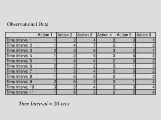
An Evaluation of Observational Data Assimilation in Alaska WRF Forecasts. Don Morton and Jing Zhang Arctic Region Supercomputing Center University of Alaska Fairbanks Fairbanks, AK 99775 [ morton|jizhang]@arsc.edu. Introduction. Case Study #2 – (Cold Start).

E N D
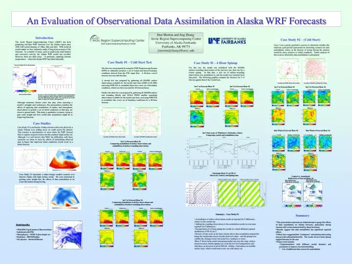
An Evaluation of Observational Data Assimilation in Alaska WRF Forecasts Don Morton and Jing Zhang Arctic Region Supercomputing Center University of Alaska Fairbanks Fairbanks, AK 99775 [morton|jizhang]@arsc.edu Introduction Case Study #2 – (Cold Start) The Arctic Region Supercomputing Center (ARSC) has been producing real-time WRF forecasts over the Alaska region since 2006 with nested domains of 18km, 6km and 2km. With archived model output we have initiated a study of long-term accuracy of the forecasts. In a number of areas, such as small-scale wind features and convective activity, the Alaska WRF model has excelled. However, there are other areas – in particular, capturing extreme temperatures – where the Alaska WRF has failed miserably. Case 2 was a purely qualitative exercise to determine whether this relatively quiet period represented an interesting scenario for data assimilation, where, in the absence of strong forcing the solution would be more sensitive to initial conditions. Future analysis of this event as affected by data assimilation is anticipated. Case Study #1 – Cold Start Test Case Study #1 – 6 Hour Spinup For this test, the model was initialized with the MADIS surface+sounding observations of the previous test, then run for a 6-hour spinup. At that time, a new set of surface+sounding observations was assimilated in, and the model was restarted from this point. The following graphics compare the forecast 2m T of this run against that of the Control run. The first test was prepared by using the WRF Preprocessing System (WPS) to ultimately produce a set of initial and lateral boundary conditions derived from the FNL input files. A 48-hour control forecast was run with this data. A second test was prepared by gathering all MADIS surface observations available for the model start time (2008-12-28_00Z) and using WRF-DA to assimilate these into a new set of boundary conditions, which was then executed for 48 forecast hours. Finally, the third test was prepared by gathering all MADIS surface and sounding (Raobs and NOAA POES satellite sounding) observations available for the model start time, and using WRF-DA to assimilate into a new set of boundary conditions for a 48-hour forecast. Locations of MADIS surface observations Locations of MADIS sounding observations 2m T at Forecast Hour 07 2m T at Forecast Hour 36 2m T at Forecast Hour 01 2m T at Forecast Hour 24 Control Surface+soundingobs Control Surface+soundingobs Control Surface+soundingobs Control Surface+soundingobs 6km resolution domain Forecast vs. Observed temperature at Fairbanks International Airport. Forecast temperature taken at Forecast Hour 12 of the daily 00Z run from July 2008 through January 2009. Note, in particular, the model’s failure to capture the extreme cold temperatures. Although numerous factors come into play when assessing a model’s strengths and weaknesses, this presentation considers the effects of applying data assimilation of surface and atmospheric observations to perturb a set of initial conditions so that they are closer to ground truth. This study is qualitative in nature, trying to gain some insight into how useful data assimilation might be in improving forecasts. Difference Difference Difference Difference Case Studies Case Study #1 is an Interior Alaska extreme cold event, driven by a classic Yakutat Low pulling arctic air south across the Interior. This scenario is representative of cases where the WRF forecast fails to capture steep inversions and the resultant frigid surface air. Although it is well known that WRF has difficulties with these scenarios, we chose to asses the effects of assimilating observed data in hopes that improved initial conditions would result in a better forecast. 10m Wind at Forecast Hour 01 10m Wind at Forecast Hour 24 2m T time series at Whitehorse, Fairbanks, Galena Comparing control and assimilation runs Control Surface+soundingobs Control Surface+soundingobs Locations of MADIS surface observations Locations of MADIS sounding observations 2m T at Forecast Hour 01 Comparing assimilation of surface observations and assimilation of surface+sounding observations Control Surface obs Control Surface+soundingobs Difference Difference Difference Difference Fairbanks Skew-T’s at FH 12 Observed, Control, and Spinup runs Case Study #2 represents a rather benign weather scenario over Interior Alaska with light surface winds. We were interested in gaining some insight into the effects of data assimilation in an event that lacked strong forcing. Control vs. Assimilated Reflectivity at Forecast Hour 24 2m T at Forecast Hour 36 Comparing assimilation of surface observations and assimilation of surface+sounding observations Control Surface obs Control Surface+soundingobs • Summary – Case Study #1 • Assimilation of surface observations results in regional 2m T differences relative to the control run • Adding the sounding observations to the assimilation results in even more regional 2m T differences • Incorporation of a 6 hour spinup also results in a much different regional distribution of FH 36 2m T • Review of time series at the three stations shows that assimilation temporarily brings the temperature down towards observed values – and the spinup case exhibits the strongest trend, but model has a tendency to warm. • Skew T shows both control and spinup model runs miss the steep, surface based inversion, but the spinup case cools the low level temperatures and introduces an inversion at about 800 mb. Further, it introduces an unstable surface layer, which would tend to mix out cold surface air. Summary • This presentation represents an initial attempt to gauge the effects of data assimilation on Alaska forecasts, particularly during extreme cold events characterized by sharp inversions • Results suggest that data assimilation has significant regional effects • Others have suggested that “continuous” assimilation and cycling may provide substantial benefits. The results of our 6-hour spinup suggest this may be the case • Future work includes • Experimentation with different model domains and parameters to improve inversion handling • Use of additional data sources for assimilation • Model Specifics • 500x500x75 grid points at 3km resolution. • Initialized with FNL • Microphysics – WSM 3-class simple ice • Radiation – RRTM/Dudhia • Sfc physics – thermal diffusion Difference Difference