Download
1 / 60
600 likes | 744 Vues
Combinatorial Aspects of Automatic Differentiation. Paul D. Hovland Mathematics & Computer Science Division Argonne National Laboratory. Group Members. Andrew Lyons (U.Chicago) Priyadarshini Malusare Boyana Norris Ilya Safro Jaewook Shin Jean Utke (joint w/ UChicago)

E N D
Combinatorial Aspects of Automatic Differentiation Paul D. Hovland Mathematics & Computer Science Division Argonne National Laboratory
Group Members • Andrew Lyons (U.Chicago) • Priyadarshini Malusare • Boyana Norris • Ilya Safro • Jaewook Shin • Jean Utke (joint w/ UChicago) • Programmer/postdoc TBD Alumni: J. Abate, S. Bhowmick, C. Bischof, A. Griewank, P. Khademi, J. Kim, U. Naumann, L. Roh, M. Strout, B. Winnicka
Funding • Current: • DOE: Applied Mathematics Base Program • DOE: Computer Science Base Program • DOE: CSCAPES SciDAC Institute • NASA: ECCO-II Consortium • NSF: Collaborations in Math & Geoscience • Past: • DOE: Applied Math • NASA Langley • NSF: ITR
Outline • Introduction to automatic differentiation (AD) • Some application highlights • Some combinatorial problems in AD • Derivative accumulation • Minimal representation • Optimal checkpointing strategy • Graph coloring • Summary of available tools • More application highlights • Conclusions
Why Automatic Differentiation? • Derivatives are used for • Measuring the sensitivity of a simulation to unknown or poorly known parameters (e.g.,how does ocean bottom topography affect flow?) • Assessing the role of algorithm parameters in a numerical solution (e.g., how does the filter radius impact a large eddy simulation?) • Computing a descent direction in numerical optimization (e.g., compute gradients and Hessians for use in aircraft design) • Solving discretized nonlinear PDEs (e.g., compute Jacobians or Jacobian-vector products for combustion simulations)
Why Automatic Differentiation? (cont.) • Alternative #1:hand-coded derivatives • hand-coding is tedious and error-prone • coding time grows with program size and complexity • automatically generated code may be faster • no natural way to compute derivative matrix-vector products (Jv, JTv, Hv) without forming full matrix • maintenance is a problem (must maintain consistency) • Alternative #2: finite difference approximations • introduce truncation error that in the best case halves the digits of accuracy • cost grows with number of independents • no natural way to compute JTv products
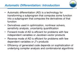
AD in a Nutshell • Technique for computing analytic derivatives of programs (millions of loc) • Derivatives used in optimization, nonlinear PDEs, sensitivity analysis, inverse problems, etc. • AD = analytic differentiation of elementary functions + propagation by chain rule • Every programming language provides a limited number of elementary mathematical functions • Thus, every function computed by a program may be viewed as the composition of these so-called intrinsic functions • Derivatives for the intrinsic functions are known and can be combined using the chain rule of differential calculus • Associativity of the chain rule leads to two main modes: forward and reverse • Can be implemented using source transformation or operator overloading
What is feasible & practical • Jacobians of functions with small number (1—1000) of independent variables (forward mode) • Jacobians of functions with small number (1—100) of dependent variables (reverse/adjoint mode) • Very (extremely) large, but (very) sparse Jacobians and Hessians (forward mode plus coloring) • Jacobian-vector products (forward mode) • Transposed-Jacobian-vector products (adjoint mode) • Hessian-vector products (forward + adjoint modes) • Large, dense Jacobian matrices that are effectively sparse or effectively low rank (e.g., see Abdel-Khalik et al., AD2008)
Application: Sensitivity analysis in simplified climate model • Sensitivity of flow through Drake Passage to ocean bottom topography • Finite difference approximations: 23 days • Naïve automatic differentiation: 2 hours 23 minutes • Smart automatic differentiation: 22 minutes
Application: solution of nonlinear PDEs • Jacobian-free Newton-Krylov solution of model problem (driven cavity) AD + TFQMR: AD + BiCGStab: FD(w=10-5 ) + GMRES: FD(w=10-3 ) + GMRES: AD + GMRES: FD(w=10-5 ) + BiCGStab: FD(w=10-7 ) + GMRES: does not converge FD + TFQMR: does not converge AD = automatic differentiation FD = finite differences W = noise estimate for Brown-Saad
Application: mesh quality optimization • Optimization used to move mesh vertices to create elements as close to equilateral triangles/tetrahedrons as possible • Semi-automatic differentiation is 10-25% faster than hand-coding for gradient and 5-10% faster than hand-coding for Hessian • Automatic differentiation is a factor 2-5 times faster than finite differences Before After
Combinatorial problems in AD • Derivative accumulation • Minimal representation • Optimal checkpointing strategy • Graph coloring
Accumulating Derivatives • Represent function using a directed acyclic graph (DAG) • Computational graph • Vertices are intermediate variables, annotated with function/operator • Edges are unweighted • Linearized computational graph • Edge weights are partial derivatives • Vertex labels are not needed • Compute sum of weights over all paths from independent to dependent variable(s), where the path weight is the product of the weights of all edges along the path [Baur & Strassen] • Find an order in which to compute path weights that minimizes cost (flops): identify common subpaths (=common subexpressions in Jacobian)
f * c * * b sin exp a y x A simple example b = sin(y)*y a = exp(x) c = a*b f = a*c
f f * a c c * a b * y b sin exp a t0 d0 a y x y x A simple example t0 = sin(y) d0 = cos(y) b = t0*y a = exp(x) c = a*b f = a*c
f a c a b y t0 d0 a y x Brute force • Compute products of edge weights along all paths • Sum all paths from same source to same target • Hope the compiler does a good job recognizing common subexpressions v5 v4 v2 v1 v3 dfdy = d0*y*a*a + t0*a*a dfdx = a*b*a + a*c V-1 v0 8 mults 2 adds
Vertex elimination • Multiply each in edge by each out edge, add the product to the edge from the predecessor to the successor • Conserves path weights • This procedure always terminates • The terminal form is a bipartite graph f a c a b
Vertex elimination • Multiply each in edge by each out edge, add the product to the edge from the predecessor to the successor • Conserves path weights • This procedure always terminates • The terminal form is a bipartite graph f a*a c + a*b
f a c a b y t0 d0 a y x Forward mode: eliminate vertices in topological order t0 = sin(y) d0 = cos(y) b = t0*y a = exp(x) c = a*b f = a*c v4 v2 v1 v3
f a c a b d1 a y x Forward mode: eliminate vertices in topological order t0 = sin(y) d0 = cos(y) b = t0*y a = exp(x) c = a*b f = a*c d1 = t0 + d0*y v4 v2 v3
f a c b d2 a y x Forward mode: eliminate vertices in topological order t0 = sin(y) d0 = cos(y) b = t0*y a = exp(x) c = a*b f = a*c d1 = t0 + d0*y d2 = d1*a v4 v3
f a d4 d2 d3 y x Forward mode: eliminate vertices in topological order t0 = sin(y) d0 = cos(y) b = t0*y a = exp(x) c = a*b f = a*c d1 = t0 + d0*y d2 = d1*a d3 = a*b d4 = a*c v4
f dfdy dfdx y x Forward mode: eliminate vertices in topological order t0 = sin(y) d0 = cos(y) b = t0*y a = exp(x) c = a*b f = a*c d1 = t0 + d0*y d2 = d1*a d3 = a*b d4 = a*c dfdy = d2*a dfdx = d4 + d3*a 6 mults 2 adds
f a c a b y t0 d0 a y x Reverse mode: eliminate in reverse topological order t0 = sin(y) d0 = cos(y) b = t0*y a = exp(x) c = a*b f = a*c v4 v2 v1 v3
f d1 d2 y t0 d0 a y x Reverse mode: eliminate in reverse topological order t0 = sin(y) d0 = cos(y) b = t0*y a = exp(x) c = a*b f = a*c d1 = a*a d2 = c + b*a v2 v1 v3
f d4 d2 d3 d0 a y x Reverse mode: eliminate in reverse topological order t0 = sin(y) d0 = cos(y) b = t0*y a = exp(x) c = a*b f = a*c d1 = a*a d2 = c + b*a d3 = t0*d1 d4 = y*d1 v1 v3
f d2 dfdy a y x Reverse mode: eliminate in reverse topological order t0 = sin(y) d0 = cos(y) b = t0*y a = exp(x) c = a*b f = a*c d1 = a*a d2 = c + b*a d3 = t0*d1 d4 = y*d1 dfdy = d3 + d0*d4 v3
f dfdy dfdx y x Reverse mode: eliminate in reverse topological order t0 = sin(y) d0 = cos(y) b = t0*y a = exp(x) c = a*b f = a*c d1 = a*a d2 = c + b*a d3 = t0*d1 d4 = y*d1 dfdy = d3 + d0*d4 dfdx = a*d2 6 mults 2 adds
f a c a b y t0 d0 a y x “Cross-country” mode t0 = sin(y) d0 = cos(y) b = t0*y a = exp(x) c = a*b f = a*c v4 v2 v1 v3
f a c a b d1 a y x “Cross-country” mode t0 = sin(y) d0 = cos(y) b = t0*y a = exp(x) c = a*b f = a*c d1 = t0 + d0*y v4 v2 v3
f d2 d3 d1 a y x “Cross-country” mode t0 = sin(y) d0 = cos(y) b = t0*y a = exp(x) c = a*b f = a*c d1 = t0 + d0*y d2 = a*a d3 = c + b*a v2 v3
f d3 dfdy a y x “Cross-country” mode t0 = sin(y) d0 = cos(y) b = t0*y a = exp(x) c = a*b f = a*c d1 = t0 + d0*y d2 = a*a d3 = c + b*a dfdy = d1*d2 v3
f dfdy dfdx y x “Cross-country” mode t0 = sin(y) d0 = cos(y) b = t0*y a = exp(x) c = a*b f = a*c d1 = t0 + d0*y d2 = a*a d3 = c + b*a dfdy = d1*d2 dfdx = a*d3 5 mults 2 adds
What We Know • Reverse mode is within a factor of 2 of optimal for functions with one dependent variable. This bound is sharp. • Eliminating one edge at a time (edge elimination) can be cheaper than eliminating entire vertices at a time • Eliminating pairs of edges (face elimination) can be cheaper than edge elimination • Optimal Jacobian accumulation is NP hard • Various linear and polynomial time heuristics • Optimal orderings for certain special cases • Polynomial time algorithm for optimal vertex elimination in the case where all intermediate vertices have one out edge
What We Don’t Know • What is the worst case ratio of optimal vertex elimination to optimal edge elimination? … edge to face? • When should we stop? (minimal representation problem) • How to adjust cost metric to account for cache/memory behavior? • Is O(min(#indeps,#deps)) a sharp bound for the cost of computing a general Jacobian relative to the function?
Minimal graph of a Jacobian (scarcity) Original DAG Bipartite DAG Minimal DAG Reduce graph to one with minimal number of edges (or smallest number of DOF) How to find the minimal graph? Relationship to matrix properties? Avoid “catastrophic fill in” (empirical evidence that this happens in practice) In essence, represent Jacobian as sum/product of sparse/low-rank matrices
Practical Matters: constructing computational graphs • At compile time (source transformation) • Structure of graph is known, but edge weights are not: in effect, implement inspector (symbolic) phase at compile time (offline), executor (numeric) phase at run time (online) • In order to assemble graph from individual statements, must be able to resolve aliases, be able to match variable definitions and uses • Scope of computational graph construction is usually limited to statements or basic blocks • Computational graph usually has O(10)—O(100) vertices • At run time (operator overloading) • Structure and weights both discovered at runtime • Completely online—cannot afford polynomial time algorithms to analyze graph • Computational graph may have O(10,000) vertices
Reverse Mode and Checkpointing • Reverse mode propagates derivatives from dependent variables to independent variables • Cost is proportional to number of dependent variables: ideal for scalar functions with large number of independents • Gradient can be computed for small constant times cost of function • Partial derivatives of most intrinsics require value of input(s) • d(a*b)/db = a, d(a*b)/da = b • d(sin(x))/dx = cos(x) • Reversal of control flow requires that all intermediate values are preserved or recomputed • Standard strategies rely on • Taping: store all intermediate variables when they are overwritten • Checkpointing: store data needed to restore state, recompute
Checkpointing: notation Perform forward (function) computation Perform reverse (adjoint) computation Record overwritten variables (taping) Checkpoint state at subroutine entry Restore state from checkpoint Combinations are possible:
Timestepping with no checkpoints 1 2 3 4 4 3 2 1
Checkpointing based on timesteps 1 2 3 4 4 3 3 2 2 1 1
Checkpointing based on timesteps: parallelism 1 2 3 4 4 3 3 2 2 1 1
Checkpointing based on timesteps: parallelism 1 2 3 4 4 3 3 2 2 1 1
Checkpointing based on timestep: hierarchical 1 2 3 4 5 6 7 8 8 7 7 6 6 5 5 1 2 3 4 4 3 3 2 2 1 1
3-level checkpointing • Suppose we use 3-level checkpointing for 100 time steps, checkpointing every 25 steps (at level 1), every 5 steps (at level 2), and every step (at level 3) • Then, the checkpoints are stored in the following order:25, 50, 75, 80, 85, 90, 95, 96, 97, 98, 99, 91, 92, 93, 94, 86, 87, 88, 89,81, 82, 83, 84, 76, 77, 78, 79, 55, 60, 65, 70, 71, 72, 73, 74, 66, 67, 68, 69, 61, 62, 63, 64, 56, 57, 58, 59, 51, 52, 53, 54, 30, 35, 40, 45, 46, … 25 50 75 100 0
Checkpointing based on call tree function split mode joint mode 1 1 1 1 1 2 2 2 2 2 2 3 3 3 3 3 3 3 Assume all subroutines have structure x.1, call child, x.2 split mode: 1.1t, 2.1t, 3.1t, 3.2t, 2.2t, 1.2t, 1.2a, 2.2a, 3.2a, 3.1a, 2.1a, 1.1a joint mode: 1.1t, 2.1, 3.1, 3.2, 2.2, 1.2t, 1.2a, 2.1t, 3.1, 3.2, 2.2t, 2.2a, 3.1t, 3.2t, 3.2a, 3.1a, 2.1a, 1.1a
Checkpointing real applications • In practice, need a combination of all of these techniques • At the timestep level, 2- or 3-level checkpointing is typical: too many timesteps to checkpoint every timestep • At the call tree level, some mixture of joint and split mode is desirable • Pure split mode consumes too much memory • Pure joint mode wastes time recomputing at the lowest levels of the call tree • Currently, OpenAD provides a templating mechanism to simplify the use of mixed checkpointing strategies • Future research will attempt to automate some of the checkpointing strategy selection, including dynamic adaptation
Matrix Coloring • Jacobian matrices are often sparse • The forward mode of AD computes J × S, where S is usually an identity matrix or a vector • Can “compress” Jacobian by choosing S such that structurally orthogonal columns are combined • A set of columns are structurally orthogonal if no two of them have nonzeros in the same row • Equivalent problem: color the graph whose adjacency matrix is JTJ • Equivalent problem: distance-2 color the bipartite graph of J
Matrix Coloring 1 2 12 0 0 5 0 0 3 0 0 0 234 0 1 0 0 0 0 0 0 0 45 12 0 5 3 0 0 0 324 0 1 0 0 0 0 0 45 5 3 1 2 0 0 5 0 0 3 0 0 0 2 3 4 0 1 0 0 0 0 0 0 0 4 5 4 1 2 12 0 0 5 0 0 3 0 0 0 234 0 1 0 0 0 0 0 0 0 45 125 0 0 3 423 1 0 0 4 0 5 5 3 4