Correspondence analysis for data mining

1. Correspondence analysis for data mining Annie Morin, IRISA France amorin@irisa.fr Jean-Hugues Chauchat, Université Lyon2, ERIC jean-hugues.chauchat@univ-lyon2.fr

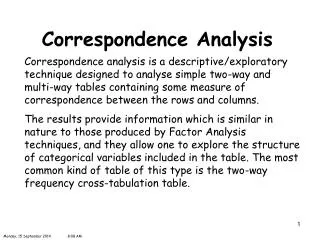
2. Correspondence analysis • Statistical visualization method for displaying the associations between the levels of a two-contingency table and the distances between the categories of each variable => exploratory method • Usually, Chi-square test for independence in a contingency table

3. 1- EXAMPLE • Data set crossing words (4 words) and 4 documents

4. Example : Frequency table

5. Questions • Explore the structure of categorical variables included in the table • Find some correspondences between the rows and columns • Well-known situation : independence between the variables defining the lines and the columns

6. How to check the independence or the relationship? • Comparison of row profiles • Comparison of column profiles • Chi-square statistics • Other indicators • CA

7. Independence situation

8. Row-profiles

9. Row-profiles

10. Column profile

11. Column-profiles

14. 2- Method • Table with r rows and c columns • nij = frequency in the cell (i,j) • ni.=nij, n.j= nij, n=  nij • Find a lower-dimensional space, in which to position the row points in a manner that retains all, or almost all, of the information about the differences between the rows (ie columns)

15. the row and column totals of the matrix of relative frequencies are called the row mass and column mass, respectively. • The term inertia is used by analogy with the definition in applied mathematics of "moment of inertia," which stands for the integral of mass times the squared distance to the centroid Inertia is defined as the total Pearson Chi-square for the two-way divided by the total sum

16. If the rows and columns in a table are completely independent of each other, the entries in the table can be reproduced from the row and column totals alone, or row and column profiles • Any deviations from the expected values (expected under the hypothesis of complete independence of the row and column variables) will contribute to the overall Chi-square. Thus, another way of looking at CA is to consider it a method for decomposing the overall Chi-square statistic (or Inertia=Chi- square/n) by identifying a small number of dimensions in which the deviations from the expected values can be represented. This is similar to the goal of FA or PCA where the total variance is decomposed, so as to arrive at a lower-dimensional representation of the variables that allows one to reconstruct most of the variance/covariance matrix of variables.

17. The dimensions are "extracted" so as to maximize the distances between the row or column points, and successive dimensions (which are independent of or orthogonal to each other) will "explain" less and less of the overall Chi-square value (and, thus, inertia ) • the maximum number of eigenvalues that can be extracted from a two- way table is equal to the minimum of the number of columns minus 1, and the number of rows minus 1

18. Plot the coordinates in a two-dimensional scatterplot. Remember that the purpose of correspondence analysis is to reproduce the distances between the row and/or column points in a two-way table in a lower-dimensional display; note that, as in Factor analysis the actual rotational orientation of the axes is arbitrarily chosen so that successive dimensions "explain" less and less of the overall Chi-square value (or inertia)

19. It is customary to summarize the row and column coordinates in a single plot. However, it is important to remember that in such plots, one can only interpret the distances between row points, and the distances between column points, but not the distances between row points and column points.

20. Quality of a displayed solution • The quality of a point is defined as the ratio of the squared distance of the point from the origin in the chosen number of dimensions, over the squared distance from the origin in the space defined by the maximum number of dimensions and is called the squared cosine

21. The relative inertia represents the proportion of the total inertia accounted for by the respective point, and it is independent of the number of dimensions chosen by the user. Note that a particular solution may represent a point very well (high quality) but the same point may not contribute much to the overall inertia

22. It should be noted at this point that correspondence analysis is an exploratory technique. Actually, the method was developed based on a philosophical orientation that emphasizes the development of models that fit the data, rather than the rejection of hypotheses based on the lack of fit (Benzecri's "second principle" states that "The model must fit the data, not vice versa;" see Greenacre, 1984, p. 10). Therefore, there are no statistical significance tests that are customarily applied to the results of a correspondence analysis; the primary purpose of the technique is to produce a simplified (low- dimensional) representation of the information in a large frequency table (or tables with similar measures of correspondence).

23. Contribution à l’inertie αème axe • Crα(i) = fi.ψ2αi/λα • ∑ contributions des individus sur un axe =1 • Qualité de la représentation :

24. Supplementary points • An important aid in the interpretation of the results from a correspondence analysis is to include supplementary row or column points, that were not used to perform the original analyses.

25. Notations • There are two clouds of points, • the first one N(I) is the set of rows whose coordinates are the components of the row profiles and the mass is the marginal frequency of the row • The second one N(J) is the set of columns whose coordinates are the components of the column profiles and the mass the marginal frequency of the column

26. Distances Between two columns Between two rows

27. Principle of distributional equivalence • If two row profiles (say) are identical the the corresponding two rows of the original matrix may be replaced by their summation (as a single row) without affecting the geometry of the column profiles.

28. CA • Duality between the row and the columns • Use of the row profiles and of the column profiles • Use of chi-square distance (distributional equivalence) • Factorial analysis method (eigen values of a ad-hoc matrix) and reduction of dimensionality

29. Diagonalization of a « covariance matrix » to find the eigenvalues and corresponding eigenvectors • λ1≥λ2≥…….. ≥λp • Inertia of the cloud is ∑λi =2 / n • Distance to the independence model

30. Simultaneous representation • Of the rows and of the columns profiles on the same factorial plane • Validity of representation : • Inertia : contributions that describe the proportion of variance explained provided by each element (row or column profile) in building an axis • Quality of representation of each element by the axes

31. Special clouds « shapes » • Guttman effect : horseshoe shape • Two sub-clouds • 3 subclouds

32. Guttman effect

33. Two sub-clouds

34. 3 sub-clouds

35. Similar techniques • Optimal scaling • Reciprocal averaging • Quantification method • Homogeneity analysis

36. Example • Initial example • Second example

38. Column coordinates

39. Column Contributions

40. Columns quality (Squared Cosine)

41. Row results

43. Second example

44. Tableau sur alcool et caractéristiques

46. Profils-lignes

47. Profils-colonnes

49. Indices d’attraction-répulsion

50. Boîtes à moustaches des dij