Download
1 / 33
330 likes | 503 Vues
Unsteady Numerical Simulation of the Turbulent Flow around an Exhaust Valve. CTU in Prague, Czech Republic 6 th – 10 th June 2011. 6 th International Symposium on Finite Volumes for Complex Applications. Unsteady Numerical Simulation of the Turbulent Flow around an Exhaust Valve.

E N D
Unsteady Numerical Simulation of the Turbulent Flow around an Exhaust Valve CTU in Prague, Czech Republic 6th – 10th June 2011 FVCA 6 6th International Symposium on Finite Volumes for Complex Applications
FVCA 6 Unsteady Numerical Simulation of the Turbulent Flow around an Exhaust Valve prof. Jaroslav FOŘT,Czech Technical University, Prague, Czech Republic prof. Herman DECONINCK,von Kármán Institute for Fluid Dynamics, Rhode-St-Genése, Belgium Milan ŽALOUDEK
FVCA 6 Outline • Motivation • Physics Solved • Numerics Used • Results • Conclusions
FVCA 6 Motivation exhaustion = complicated issue physical – determined by many factors (unsteady, 3D, turbulent, chemistry, ...) numerical – see later difficult comparisons of results one of the least explored engine domains hardly no experimental data doubtful results from comercial CFD codes exhaust valve and exhaust pipe sudden area widenings and restrictions sharp corners causing flow separation wide velocity range goal: insight of the flow structure
FVCA 6 Physics Solved
FVCA 6 Flow characteristics during real operating cycle fully 3D flow exhaust valve opens and closes very quickly turbulent flow, possibly involving some chemistry problems of numerical solution moving boundaries unsteady flow conditions wide velocity range formulation of outlet boundary condition (recirculation zone leaving and re-entering the domain) velocity streamlines Mach number ilustrating solution, one half of the valve contour
Governing Equations conservative variables • Reynolds-Averaged Navier-Stokes equations convective fluxes viscous fluxes source term ρdensity, (w1,w2) velocity components, p pressure, e internal energy, T temperature, k turbulent kinetic energy, ω specific dissipation rate stress tensor heat fluxes • constitutive relations closing the set of equations equation of state, Sutherland’s law, Fourier’s law FVCA 6
Turbulence Modelling • main variables decomposed to mean part and fluctuation part • density weighted averaging, suitable for compressible flows • Boussinesq hypothesis – analogy between molecular and turbulent transport of momentum • Reynold’s stress tensor • turbulent viscosity extracted from turbulence model Models implemented and used • Menter’s baseline model (BSL) • Wilcox k-ω model, rev. 2008 • Explicit Algebraic Reynolds Stress Model (EARSM) FVCA 6
Menter’s BSL model (1994) • transport eq. for turbulent kinetic energy k and specific dissipationω • blending between k-ωmodel near walls and k-εmodel in freestream • transport equations ofεadded through blending function F1 • turbulent viscosity • model constants combined via k-ω: k-ε : FVCA 6
Wilcox’s k-ω model (2008) • transport eq. for turbulent kinetic energy k and specific dissipationω • limiting magnitude of turbulent viscosity • cross-diffusion term • model constants FVCA 6
Wallin’s EARSM (2000) • explicit algebraic Reynolds stress model • non-linear relation for turbulent stresses with respect to Sij • turbulent viscosity • anisotropy term • normed tensors • turbulent time-scale • transport eq. for k and ωin a form of Kok’s TNT k-ωmodel • coefficients • model constants FVCA 6
Mathematical Formulation • W fulfils equation • W fulfils initial condition and boundary conditions • searching for a function W(xi, t), on a domain Ω such that FVCA 6
Mathematical Formulation • Boundary conditions • Inlet: total pressure, total temperature, incidence angle, turb. variables • Outlet: pressure, velocity, temperature, turbulent variables • Wall: no-slip condition, turb. variables according to literature (F.R. Menter) • Symmetry: non-permeability condition • Computational domain FVCA 6
FVCA 6 Numerics Used
Numerical Solution Computational Object Oriented Library for Fluid Dynamics • in-house CFD code COOLFluiD • developed by group of engineers, based at VKI • based on finite volume method (FVM) • cell-centered approach, variables stored in centroids of each cell • continuous problem discretized with the Gauss theorem • explicit or implicit time integration • spatial accuracy improved by a linear reconstruction (obtained by a least squares interpolation method) and the Barth limiter • the arbitrary Lagrangian-Eulerian (ALE) formulation used for unsteady flow simulations • time accurate computations using Crank-Nicholson scheme and/or backward differentiation formula (BDF2) FVCA 6
Implicit Time Integration • steady flow computation • original equation transforms to • J Jacobian matrix, ΔW difference in vector of unknowns, R right hand side (time dependent terms, numerical fluxes, source terms) • linear system solved by GMRES iterative solver (provided by PETSc) • Jacobian matrix computed numerically • unsteady flow computation • dual time stepping • outer t.s. (Δt) – real time accurate step, 1st step C-N, further on BDF2 • inner t.s. (Δτ) – solving the system at each real time step • linear system solved by GMRES FVCA 6
Convective Fluxes • AUSM+up, Advection Upstream Splitting Method, modified for all speeds • based on solution of Riemann problem – flux over 1D discontinuous step between two states WL, WR • MLR, pLR computed using splitting polynoms, ΦLR upwinded • Mcorr, pcorr corrections to ensure better convergence at low speeds FVCA 6
Convective Fluxes • Mcorr, pcorr corrections to ensure better convergence at low speed • M∞ freestream Mach number, affect correction terms through fa FVCA 6 inviscid flow in a channel, solved with numerical scheme without (left), with (right) corrections sequence for different freestream velocities M=0.020, M=0.200, M=0.675 (top to bottom)
Viscous Fluxes Source Terms • computed by a central approximation • using diamond dual cells • derivatives computed by the Gauss theorem • evaluated cell-wise Computational Grids • structured triangular grids (splitted quadrilaterals) • due to large grid displacements, unsteady flow simulations employ set of grids for different valve lifts • solution between grids interpolated by the Shepard method FVCA 6
FVCA 6 Results
Flow Structure (1/3) • steady flow computation • 2D, turbulent flow model (BSL) • valve opening 4 mm • temperature 500 K • pressure ratio contours of Mach number FVCA 6
Flow Structure (2/3) detail of outlet boundary detail of valve seat outlet maximal M = 1.12 average M = 0.72 no backflow supersonic expansion around corner shock waves deflecting flow causing separations on both sides overall max M = 2.85 artificial channel throat determined by recirculations allowing further expansion FVCA 6
Flow Structure (3/3) detail bottom corner detail of expansion separation behind valve seat separation at corner, where valve meets its casing separation behind the pipe corner separation along the exhaust valve separation on a straight wall FVCA 6
Influence of Turbulence Model (1/3) • 2D model • steady flow computation • identical boundary conditions • valve opening 4 mm • pressure ratio pin/pout = 2.5 (exhaust to atmosphere) • temperature 500 K • qualitative agreement of all models • BSL and Wilcox model very close • EARSM predicts different flow topology FVCA 6 contours of Mach number
Influence of Turbulence Model (2/3) Comparison of pressure and Mach number throughout pipe • data extracted along (main) streamline passing through the middle of the channel throat • BSL, Wilcox models almost identical • EARSM holds trend, but predicts milder peaks and higher outlet velocity FVCA 6
Influence of Turbulence Model (3/3) Positions of separation zones • zero coordinates at channel throat (aerodynamically choked) • distances in milimeters FVCA 6
Unsteady Flow Simulation (1/5) • 2D, turbulent flow model (BSL) • movement corresponds to RPM = 3.500, one valve loop ≈ 1.5 10-2 s • boundary conditions set according to the literature (J. Heywood) • various inlet pressure evolution - spark ignition / compression ignition • same outlet pressure evolution • max. valve lift 11 mm, treshold 0.5 mm • time step Δt = 10-6 s • computational grids for different lifts: 0.5 – 2.5 – 7.0 mm • remeshing + interpolation points FVCA 6
Unsteady Flow Simulation (2/5) Spark ignition (SI) engine • valve loop ≈ 1.5 10-2 s, time step Δt = 10-6 s • step solution displayed Δt = 10-4 s • see full movie FVCA 6
Unsteady Flow Simulation (3/5) Compression ignition (CI) engine • valve loop ≈ 1.5 10-2 s, time step Δt = 10-6 s • step solution displayed Δt = 10-4 s • see full movie FVCA 6
Unsteady Flow Simulation (4/5) Comparison of un-steady approach • valve lift 7.0 mm • inlet BC corresponds to CI engine (closing phase) • Mach number contours • pressure evolution in exhaust pipe unsteady solution steady solution FVCA 6
Unsteady Flow Simulation (5/5) Mass flow comparison • CI engine detects higher ṁ, due to higher operating pressure ratio • ṁ coincides in early stages for both engines, due to aerodynamical choking • ṁ at very low lifts negligible • differences against steady solutions approx. ≈ 10% mass flow rate [kg/s] FVCA 6
FVCA 6 Conclusions reasonable results of gas exhaustion acquired with in-house developed CFD code (respecting physical assumptions) gas exhaustion phenomena even small geometrical difference cause dramatic flow changes careful capturing of separation zones required exhaustion unsteadiness can not be neglected final target: insight of the flow topology Future Prospects • more turbulence models for unsteady flow computations • extension to 3D unsteady computations • optimization of the exhaust valve shape • complete simulation of a 4-stroke engine (cylinder domain)
FVCA 6 Acknowledgements This work has originated thanks to team of patient co-workers developers of CFD package COOLFluiD grant GAČR No. P101/10/1329 Josef Božek Research Center 1M6840770002