Download

1 / 40
460 likes | 865 Vues
STA 107: Logistic Regression and Categorical Data Analysis . Lecturer: Dr. Daisy Dai Department of Medical Research. Contents . Binary Logit Analysis Simple Logistic Regression Multiple Logistic Regression Stepwise or Backward Model Selections Collinearity. Categorical Data Analysis.

E N D
STA 107: Logistic Regression and Categorical Data Analysis Lecturer: Dr. Daisy Dai Department of Medical Research
Contents • Binary Logit Analysis • Simple Logistic Regression • Multiple Logistic Regression • Stepwise or Backward Model Selections • Collinearity
Categorical Data Analysis Binomial Test Chi-square Test Fisher’s Exact Test McNemar’s Test Cochran-Mantel-Haenszel Test
Binomial test Make inference about a proportion of binary outcomes by comparing the confidence interval of a proportion to target.
Case Study: Genital Wart • A company markets a therapeutic product for genital warts with a known cure rate of 40% in the general population. In a study of 25 patients with genital warts treated with this product, patients were also given high doses of vitamin C. As shown in Table on the next page, 14 patients were cured. Is this consistent with the cure rate in the general population?
Results • 64% (16/25) of patient were cured by the treatment. • The 95% confidence interval extends from 44% to 80% • If the probability of "success" in each trial or subject is 0.300, then the chance of observing 16 or more successes in 25 trials is 0.045 (p-value). • The cure rate of genital wart by the experimental therapy was significantly higher than 30%.
Fisher’s Exact Test A conservative non-parametric test about a relationship between two categorical variables. The groups in comparison should be independent.
Case Study: CHF Incidence A new adenosine-releasing agent (ARA), thought to reduce side effects in patients undergoing coronary artery bypass surgery (CABG), was studied in a pilot trial. Fisher’s exact test: p=0.0455
Chi-square test Test a relationship between two categorical variables. Groups should be independent. The chi-square test assumes that the expected value for each cell is five or higher.
Case Study: ADR Frequency with Antibiotic Treatment A study was conducted to monitor the incidence of GI adverse drug reactions of a new antibiotic used in lower respiratory tract infections. Chi-square test: p=0.0252; Fisher’s exact test: p=0.0385
McNemar’s test Compare response rates in binary data between two related populations. It’s analogous to Chi-square test or Fisher’s exact test for independent populations.
Case Study: Bilirubin A study was conduct to evaluate the toxicity side effect of an experimental therapy. Patients (n=86) were treated with the experimental drug for 3 months. Clinical lab measured bilirubin levels of each patient at baseline and 3 months after therapy.
Results of McNemar’s Test • At baseline, 14% (12/86) of patients had abnormally high bilirubin level. • At 3 months post treatment, 23% (20/86) of patients had abnormally high bilirubin level. • P-value = 0.1175 • Odds ratio = 2.3; 95% CI: 0.8 - 7.4 • There is no enough evidence to prove the increasing risk of high bilirubin due to treatment.
Cochran-Mantel-Haenszel (CMH) Test • The Cochran-Mantel-Haenszel test is a method to compare the probability of an event among independent groups in stratified samples. • The stratification factor can be study center, gender, race, age groups, obesity status or disease severity. These underlying sub-population can be confounding factors that affect the associations between risk factors and the outcome variables.
Case Study: Diabetic Ulcers • A multi-center study with 4 centers is testing an experimental treatment, Dermotel, used to accelerate the healing of dermal foot ulcers in diabetic patients. Sodium hyaluronate was used in a control group. Patients who showed a decrease in ulcer size after 20 weeks treatment of at least 90% surface area measurements were considered ‘responders’. The numbers of responders in each group are shown in Table 19.2 for each study center. Is there an overall difference in response rates between the Dermotel and control groups?
The interest in this study is to compare the response rate between two treatment. Because the study was conducted in four centers, it is concerned that some potential influences of study center on the response rate. By including the study center, the researcher can examine associations between the treatment and the response rate while adjusting (controlling) for the effect of study center. • Cochran-Mantel-Haenszel Test assumes a common odds ratio and test the null hypothesis that the explanatory variable X (treatment) and the outcome variable Y (response rate) are conditionally independent, given the control variable Z (study center). In other words, CMH tests whether the response is conditionally independent of the explanatory variable when adjusting for the control variable. • One can also measures average conditional association between the explanatory (treatment) and the response variable by calculating the common odds ratio conditioned on the control variable (study center).
Results *P-value from CMH test
Chi-Square Test, Ignoring Strata Chi-square value = 3.798, p = 0.051 p. 313
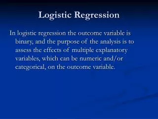
Logistic Regression • Logistic Regression are methods to identify the associations between a categorical outcome variable and explanatory variables. • In most cases, the outcome variable is dichotomous. The explanatory variables can be categorical or continuous. The probability of the outcome variable can be predicted by the values of explanatory variables. Dichotomous outcome variable explanatory variables Log(P/(1-P))=a + b1 * x1 + b2 * x2 + b3 * x3 + b4 * x4+…
Odds Ratio • Let Y be the dichotomous variable where y=1 indicates an event and y=0 indicates no events • Odd=probability of an event/probability of no event =P(Y=1)/P(Y=0)=P(Y=1)/(1-P(Y=0)) • Odds Ratio=Odds in the Test Group/Odd in the Control Group • Logistic Model: Log(Odds Ratio of an event) explanatory variables • Log (odds ratio)=a + b1 * x1 + b2 * x2 + b3 * x3 + b4 * x4+…
A new adenosine-releasing agent (ARA), thought to reduce side effects in patients undergoing coronary artery bypass surgery (CABG), was studied in a pilot trial. Odd of CHF incidence in the ARA group=(2/35)/(33/35)=2/33=6%. Odd of CHF incidence in the Placebo group=(5/25)/(20/25)=20%. Odds Ratio=Odd in the ARA group/odd in the Placebo group=(2/33)/(5/20)=0.24 The risk (odd) of CHF incidence in the ARA group is only 24% the risk (odd) in the Placebo group. Case Study: CHF Incidence Fisher’s exact test: p=0.0455
Properties of Odds Ratio • Odds ratio is non-negative. • If odds ratio<1, then the risk is smaller than control. • If odds ratio>1, then the risk is larger than control. • Odds ratio of no event=1/odds ratio of an event. • One can calculate the confidence interval of an odds ratio. The confidence interval of a significance odds ratio does not contain 1.
A new adenosine-releasing agent (ARA), thought to reduce side effects in patients undergoing coronary artery bypass surgery (CABG), was studied in a pilot trial. odds Ratio for ARA versus Control=(2/33)/(5/20)=0.24<1. So the risk of CHF incidence in the ARA group is relatively smaller. One can also calculate odds ratio for Control versus ARA as 1/0.24=4.1>1, which indicates the risk (odd) of CHF in Placebo group is 4.1 fold of risk in ARA group. Case Study: CHF Incidence Fisher’s exact test: p=0.0455
Logistic Probability Curve • Log(p/(1-p))=a+bx • p/1-p=exp(a+bx) • p=1/(1+exp(-a-bx)) Probability X
In linear regression the dependent variable is continuous The relationship is summarized by a regression equation consisting of a slope and an intercept. In increases with unit increase in the independent variable, and the intercept represents the value of the dependent variable when the independent variable takes the value zero. in logistic regression the dependent variable is binary. In logistic regression the slope represents the change in log odds for a unit increase in the independent variable and the regression we are interested in the simultaneous relationship between one dependent variable and a number of independent variables. Logistic Regression vs. Linear Regression Common: In regression we are looking for a dependence of one variable, the dependent variable, on other, the independent variable(s).
Case Study: Relapse Rate in AML One hundred and two patients with acute myelogenous leukemia (AML) in remission were enrolled in a study of a new antisense oligonucleotide (asODN). The patients were randomly assigned to receive a 10-day infusion of asODN or no treatment (Control), and the effects were followed for 90 days. The time of remission from diagnosis or prior relapse (X, in months) at study enrollment was considered an important covariate in predicating response. The response data are shown in next page with Y=1 indicating relapse, death, or major intervention, such as bone marrow transplant before Day 90. Is there any evidence that administration of asODN is associated with a decreased relapse rate?
Effect Selection Methods Statistical model selection will facilitate selection and screening of explanatory variables from a sets of candidate variables. The commonly used model selection method include: • Backward selection: starting with all candidate variables and testing them one by one for statistical significance, deleting any that are not significant. • Forward selection: starting with no variables in the model, trying out the variables one by one and including them if they are 'statistically significant'. • Stepwise selection: A combination of both methods. Select a most significant variable from the candidate pool and remove this variable if it’s not significant in the joint model. And repeat this process step by step for all remaining variables.
Multicollinearity • Multicollinearity occurs when two or more explanatory variables in a multiple regression model are highly correlated. In other words, there is redundant explanatory variables in the multiple regression models. • Multicollinearity can cause problematic estimate in the individual effects. A high degree of multicollinearity can also cause computer software packages to be unable to perform the matrix inversion that is required for computing the regression coefficients, or it may make the results of that inversion inaccurate. • Note that in statements of the assumptions underlying regression analyses such as ordinary least squares, the phrase "no multicollinearity" is sometimes used to mean the absence of perfect multicollinearity, which is an exact (non-stochastic) linear relation among the regressors.
Detection of Multicollinearity • Large changes in the estimated regression coefficients when a predictor variable is added or deleted • Tests of the individual effects of affected variables are not significant, but a global test of overall model is significant (using an F-test). • Use variance inflation factor (VIF) to detect multicollinearity: Regress a explanatory variable on all the other explanatory variables. A high coefficient of determination, r2, indicates the regressed explanatory variable was highly corrected with other explanatory variables. A tolerance=1-r2. VIF=1/tolerance. A tolerance of less than 0.20 or 0.10 or a VIF of 5 or 10 and above indicates a multicollinearity problem.
Caveats • Sometimes logistic regression is carried out when a dependent variable is dichotomized. It is important that the cut point is not derived by direct examination of the data for example to find a ‘gap in the data which maximizes the discrimination between the selected groups as this can lead to biased results. It is bests if there are a priori grounds for choosing a particular cut point.
References • Common Statistical Methods for Clinical Research 2nd Edition by Glenn Walker • Logistic Regression Using The SAS System by Paul Allison • Medical Statistics by Campbell et al.