Download
1 / 21
210 likes | 365 Vues
THE AGGREGATE DEMAND/ SUPPLY MODEL. The U.S. Great Depression. 1929-1939 Output fell by 30% Unemployment as high as 25% Prices declined 30% in the first four years Led to the development of modern macroeconomic theory Video. Before: Classical Economics.

E N D
The U.S. Great Depression • 1929-1939 • Output fell by 30% • Unemployment as high as 25% • Prices declined 30% in the first four years • Led to the development of modern macroeconomic theory Video
Before: Classical Economics • Focused on long-run issues--growth • Self-regulating markets through the “invisible hand” • Prices would adjust during recessions • Economy would always return to its potential output in the long-run • Depression caused by institutions that prevented prices from falling, specifically: • Labor unions • Government • Advocated a laissez-faire (hands-off) economic policy
After: Keynesian Economics • John Maynard Keynes in The General Theory of Employment, Interest, and Money (1936) • Problems of the Depression required a short-run, rather than long-run, focus.
Keynesian Economics • Adjustments to equilibrium for a single market and the aggregate economy are different. • Short-run equilibrium income may differ from long-run potential income. • Paradox of thrift • In long run, saving leads to investment and growth. • In short run, saving may lead to a decrease in spending, output, and employment. • Aggregate demand management by government may be necessary.
Keynesian Economics and the AS/AD Model • Aggregate Demand Curve (AD) • Relates changes in the price level to changes in aggregate expenditures = C + I + G + (X-M) • Short-Run Aggregate Supply Curve (SAS) • Relates changes in the price level to changes in aggregate supply. • Long-Run Aggregate Supply Curve (LAS) • Shows potential output at any point in time
Multiplier effect The Aggregate Demand Curve Price level Wealth, interest rate, and international effects P0 P1 AD Y0 Y1 Ye Real output
200 100 AD1 Shifts in the AD Curve Initial effect = 100 increase in expenditures Price level Multiplier effect = 200 Change in total expenditures = 300 P0 AD0 Real output
The Short-Run Aggregate Supply Curve SAS Price level Real output
Shifts in the SAS Curve 1. Higher input prices SAS1 2.Higher import prices 3. Higher sales and excise taxes Price level 4. Reduced productivity SAS0 Real output
LAS1 Long-Run Aggregate Supply Curve LAS • LAS curve shows potential output • Vertical because potential output • is unaffected by the price level. Price Level • Increases in capital, resources, • growth-compatible institutions, • technology, and entrepreneur- • ship increase potential output • and shift LAS to the right. Potential output Real output
LAS Curve LAS • Potential output is assumed to be the • middle of a range bounded by high • and low levels of potential output. C • When resources are over-utilized • (point C), factor prices may be bid • up • When resources are under-utilized • (point A), factor prices may be bid • down B A SAS Price Level Underutilized resources Overutilized resources • When LAS = SAS (point B), there is • no pressure for prices to rise or fall. Real output Low-level potential output High-level potential output
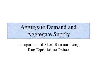
P1 F P0 E AD1 AD0 Y1 Y0 Short-Run Equilibrium:Changes in AD • Short-run equilibrium is • where SAS = AD0 (point • E). Price level • If AD increases to AD1, • equilibrium output • increases to Y1 and the • price level increases to P1. SAS P0 E AD0 Y0 Real output
SAS1 G P1 E P0 Y1 Short-Run Equilibrium:Changes in SAS • Short-run equilibrium is • where SAS0 = AD (point • E). Equilibrium output is • Y0 and the price level is • P0. Price level SAS0 • If SAS increases to SAS1, • equilibrium output • decreases to Y1 and the • price level increases to P1 • (point G). E P0 AD Y0 Real output
H P1 AD1 Long-Run Equilibrium LAS Price level • Long-run equilibrium is • point E where AD0 = LAS. • Equilibrium output is at • potential output YP and • the price level is Po. E P0 • An increase in AD to AD1 • increases the price level • to P1 but output is un- • changed at YP. AD0 YP Real output
Integrating Short-Run and Long-Run Frameworks • The economy is in long-run and short-run equilibrium at point E where AD=SAS=LAS and output is YP and the price level is P0. LAS SAS E Price level • AD grows at the same rate as potential output, so that unemployment and inflation are very low. P0 AD YP Real output
SAS0 A P0 Y1 Recessionary Gap • A recessionary gap is the amount by which equilibrium output is below potential output. LAS • At point A, some resources are unemployed and the recessionary gap is YP – Y1. SAS0 A P0 Price level AD Recessionary gap Y1 YP Real output
Inflationary Gap • An inflationary gap is the amount by which equilibrium output is above potential output. LAS Price level • If the economy is at point C, resources are being used beyond their potential and the inflationary gap is Y2 – YP. C SAS0 P0 AD Inflationary gap YP Real output Y2
B P1 AD1 YP Expansionary Fiscal Policy Price level • Economy is at equilibrium at A, there is a recessionary gap Y0 – YP. LAS • Appropriate fiscal policy is to increase government spending and/or decrease taxes. SAS P0 A A • AD increases to AD1 and output returns to potential output YP and prices increase slightly to P1. AD0 Y0 Real output
AD2 Contractionary Fiscal Policy LAS • Economy is at equilibrium at B, there is an inflationary gap Y2 – YP. • Appropriate fiscal policy is to decrease government spending and/or increase taxes. B AS P2 Price level AD0 • AD0 decreases to AD2 and output returns to potential output YP and inflation is prevented. YP Y2 Real output
Macro Policy Problems • Implementing fiscal policy • Slow legislative process • Slow and uncertain reaction by the economy • Avoiding “over-correcting”