Download
1 / 53
530 likes | 673 Vues
Integrated Population Modeling a natural tool for population dynamics. Jean-Dominique LEBRETON CEFE, CNRS, Montpellier, France jean-dominique.lebreton@cefe.cnrs.fr. INTRODUCTION Demog. & census info, the Greater snow goose Model trajectory vs census STATE SPACE MODELS State equation

E N D
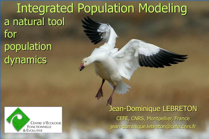
Integrated Population Modelinga natural tool for population dynamics Jean-Dominique LEBRETON CEFE, CNRS, Montpellier, France jean-dominique.lebreton@cefe.cnrs.fr
INTRODUCTION • Demog. & census info, the Greater snow goose • Model trajectory vs census • STATE SPACE MODELS • State equation • Observation equation • State-space model • FITTING STATE SPACE MODELS • The Kalman filter, Kalman smoother • « Integrated » likelihood • Normal approximation • BACK TO THE GREATER SNOW GOOSE
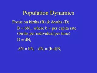
1.Demographic and census information • Changes in numbers tell us something about population mechanisms • Demographic information (e.g., CR data + statistical model) used to understand "what happened" • More precisely • Census or surveys can be used to estimate rate of population change • A "dynamic model" is needed to translate demographic estimates into estimates of rate of population change • The two types of estimates of rate of change are compared • The model can be modified and parameter estimates “tuned”
Migration stopover in spring and autumn along Saint-Laurent The Greater Snow Goose Anser caerulescens atlantica : the eastern population of snow goose Breeds eastern arctic Canada islands Winters mostly near Cheasapeake bay
The GSG: a real world problem « Why we need go on spring hunting »
Leslie Matrix Model Age-dep. breeding Prop. * fecund. * 1st year survival a3*f*s1 f*s1 0 0 ¤ ¤ ¤ 0 0 0 0 ¤ 0 0 0 0 ¤ ¤ Age - dependent survival Population Projections
Leslie Matrix Model Age-dep. breeding Prop. * fecund. * 1st year survival a3*f*s1 f*s1 0 0 ¤ ¤ ¤ 0 0 0 0 ¤ 0 0 0 0 ¤ ¤ Age - dependent survival Population Projections Harvest
Capture-recapture analysis: Survival of GSG with winter harvest as a covariate High harvest low survival slow growth or decrease
2. Model trajectory vs censussurvival driven by harvest (+ further time-dependent parameters) Year 73 74 … i i+1 … 2002 Harvest x73 x74 … xi xi+1 ... x02 Survival 73 74 ... ii+1 ... 02 Matrix M73 M74 ... Mi Mi+1 ... M02 Numbers obtained by a « time-varying matrix model » (using N73 based on average stable age structure): Ni+1=M(i)*Ni
2. Model trajectory vs censussurvival driven by harvest (+ further time-dependent parameters)
2. Model trajectory vs censussurvival driven by harvest (+ further time-dependent parameters) « tuning »: S’=1.07*S
What do we need ? • Better integration of demographic information and survey information (rather than "ad hoc" comparison) • Structured models (Matrix models in practice) should play a central role • Usually census less detailed than vector used in model • Strong need for adequate methodology in relation with "integrated monitoring" (census + marked individuals) • Methodology must be probabilistic for estimation, model selection, etc…
INTRODUCTION • Demog. & census info, the Greater snow goose • Model trajectory vs census • STATE SPACE MODELS • State equation • Observation equation • State-space model • FITTING STATE SPACE MODELS • The Kalman filter, Kalman smoother • « Integrated » likelihood • Normal approximation • BACK TO THE GREATER SNOW GOOSE
3. State equation A linear (Markov) model for a state vector = Matrix model, Greater snow goose
General form (Harvey 1989, p. 101) First order Markov Process at = Ttat-1 + ct + Rtt Tt is a m x m matrix ct is a m x 1 matrix Rt is a m x g matrix (optional) t is a g x 1 matrix of random deviations, E(t)=0 var(t)=Qt cov(t-1, t)=0
State equation: change over time • at = Ttat-1 + ct + Rt t • Tt, ct and Rt are "system matrices" • They may change with time in a predetermined way only • Only quantities in greek symbols are random variables
State equation In population applications: at = Ttat-1 + ct + Rt t often reduces to at = Tt() at-1 + t i.e., ct =0 and Rt = Id Tt() will be in a first step considered as known, i.e. the parameters are supposed to be known, i.e. one works conditional on the parameter values
Initial value The system starts with values provided for E(a0) = a0 var(a0)=P0 Cf the calculation of N73 for the GSG Usually easy and not critical
et : what stochasticity? For survival : binomial For fecundity: Poisson i.e. Demographic stochasticity All can be easily approximated by Normal distributions,in particular for large population sizes
4. Observation equation In the case of the snow goose, one observes the total spring (pre-breeding population) y(t) = Ni(t) + t = (1 1 1 1) N(t)+ t More generally, Yt can be a vector (examples later)
General form Yt = Ztat + dt + t Zt is an N x m matrix (i.e. Yt can be a vector) dt is an N x 1 matrix t is a N X 1 random matrix, E(t)=0, var (t)=Ht As previously, the system matrices Zt and dt can only change over time in a predetermined way Often Zt is constant, and dt=0, i.e. the observation equation reduces to: Yt = Z at + t
5. State-space model • A state-space model is the combination of: • A state equation (SE) at = Tt()at-1 + ct + Rtet • An observation equation (OE) Yt = Ztat + dt + t • Only YT= (Y1, Y2 , ...,YT) is observed • Under the assumptions above, everything is linear • Normal distributions for ht, et, a0 Normal distributions for at, Yt, t = 1,...,T (by linearity)
A classical exampleSatellite tracking State equation : dynamical model for the coordinates (x y z) of a satellite, based on Kepler's laws etc... Observation equation: distances to ground stations converted into coordinates measured with error Purpose: estimate (x y z) at any time based on all the information available (present and past + constraints induced by the movement model (SE))
Greater Snow Goose = state equation (Leslie matrix) Observation equation for the pre-breeding census of the total population = y(t) = Ni(t) + t = (1 1 1 1) N(t)+ t How to combine the information brought by the survey and that brought by capture-recapture analyses on the parameters in the Leslie matrix ?
INTRODUCTION • Demog. & census info, the Greater snow goose • Model trajectory vs census • STATE SPACE MODELS • State equation • Observation equation • State-space model • FITTING STATE SPACE MODELS • The Kalman filter, Kalman smoother • « Integrated » likelihood • Normal approximation • BACK TO THE GREATER SNOW GOOSE
7. The Kalman filter For a state space model at = Tt()at-1 + ct + Rt et Yt = Ztat + dt + ht • One may wish to estimate: • the state vector at, based on Yt (filtering) • the states vectors a1,..., aT, based on YT (smoothing) • the parameters (with little hope of estimating them all because of the usual loss of dimension from at to Yt)
for the state-space model at = Tt()at-1 + ct + Rt et and Yt = Ztat + dt + ht with only YT= (Y1, Y2 , ...,YT) observed • The prob. density of YT can be expressed as: • f(YT)={Pt=2,...T f(Yt | Yt-1, a0, ) } f(Y1 | a0, )g(a0) • By linearity, normal distributions for et and ht lead to normal distributions for at and Yt • We just need expectations and covariance matrices to be able to set up a likelihood • The Kalman filter is a set of recurrence relationships for expectations and covariance matrices
Linearity and normal distributions • By linearity, normal distributions for et and ht lead to normal distributions for at and Yt • ... thanks to the lemma: • X | m N(m,SX) and m N(m,V) X N(m, SX + V) • Non-normality implies tedious, often impractical, integrations • Monte-Carlo Markov Chain (MCMC) Bayesian algorithms can be viewed as stochastic integration algorithms
Filtering for the state-space model at = Tt()at-1 + ct + Rt et and Yt = Ztat + dt + ht with covariance matrices var(ht)=Qt and var(et)=Ht Using var(AX)=A var(X) A' and other classical properties • Initial conditions: a0 N(a0, P0) • Apply the SE, conditional on information at time 0: a1 N(a 1|0 + c1, P1|0) with a 1|0 = T1a0+c1 and P1|0 = T1P0T1' + R1Q1R'1 • Rearrange the SE and OE: a1 = a1|0 + (a1-a1|0) • Y1=Z1a1|0+d1+Z1(a1-a1|0)+1
Filtering From a1 N(a 1|0 + c1, P1|0) a1 = a1|0 + (a1-a1|0) Y1=Z1a1|0+d1+Z1(a1-a1|0)+1 a1 a1|0 P1|0 P1|0 Z1' N , Y1 Z1a1|0+d1 Z1P1|0 Z1P1|0 Z1'+H1 Get distribution of a1 conditional on Y1 by multiple regression
XmXsXXsXY YmYsYXsYY N , X | Y = N( mX-sXYsYY-1(y-mY),sXX-sXYsYY-1sYX) E(X | Y) corresponds to DX|Y
Lemma: multiple regression • X mXSXXSXY • N , • Y mY SYX SYY • The distribution of X conditional on Y is: • X | Y N (mX + SXY SYY-1 (Y-mY) , SXX - SXY SYY-1 SYX)
Filtering From a1 a1|0 P1|0 P1|0 Z1' N , Y1 Z1a1|0+d1 Z1P1|0 Z1P1|0 Z1'+H1 a1 | Y1 N ( a1, P1) , with a1 = a1|0 + P1|0Z1' F1-1 (Y1-Z1a1|0-d1) P1 = P1|0 - P1|0Z1' F1-1 Z1'P1|0 where F1 = Z1P1|0 Z1' + H1 .... go on over time with the same recursion to getat | Yt
Filtering • E(at | Yt) is also the Minimum MSE Estimate of at • In passing the distribution of Yt|t-1 is obtained (as was that of Y1 conditional on the information at time 0) • Hence f(Yt | Yt-1, a0, ) and the likelihood can be produced • E(at | Yt ) is a prediction based on the past, well adapted to dynamical systems in real time (prediction of the coordinates of a satellite based on the info available at time t) • E(at | YT ), based on all info before and after t, will be more relevant in general to population dynamics models
Smoothing • E(at | YT ), based on all info before and after t, will be more relevant in general to population dynamics models • It will be also more precise than E(at | Yt ), that may be useful for predictions one-step ahead • Estimation of at by E(at | YT ) is called "smoothing" • Estimation of a single at is based "fixed-point smoothing" • May be useful to estimate missing values • Estimation of all at = "interval smoothing" • Based on backwards recursions starting from T
Smoothing • Start from aT|T = aT and PT|T = PT obtained from the KF • iterate • a t|T = at+Pt* (at+1|T-Tt+1at) • Pt|T = Pt + Pt*(Pt+1|T-Pt+1|t)Pt*' • Pt* = PtTt+1' Pt+1|t-1 • Proof involved • Produces Minimum MSE estimators, in particular of state vector
7. « Integrated » Likelihood • Traditional use of Log LC(Y,) conditional on : • Estimate state vectors at • Non traditional use (Morgan et al.): based on independence, combine with capture-recapture Log-Likelihood Log LR(CR-Data, ) as: • Log LR(CR-Data, ) + Log LC(Y,) • Estimate using all info (CR + Census) • Estimate variance of census • Estimate state vectors at • Estimate pop size using all info (CR + Census)
8. Normal approximation • Integration as Log LR(CR-Data, ) + Log LC(Y,) is difficult in practice, because the first term is involved • Specific Matlab code (Besbeas et al.) • Specific program (integrated M-SURGE ?) • Simplify calculations of Log LR(CR-Data, ): approximation based on MLEs asympt.distribution • N (, S), replacing S by estimate S • Log LR(CR-Data, ) -(n log(2p)+log(det S) )/2-( - )'S-1( - )/2 (approx. of deviance by paraboloid tangent at MLE)
INTRODUCTION • Demog. & census info, the Greater snow goose • Model trajectory vs census • STATE SPACE MODELS • State equation • Observation equation • State-space model • FITTING STATE SPACE MODELS • The Kalman filter, Kalman smoother • « Integrated » likelihood • Normal approximation • BACK TO THE GREATER SNOW GOOSE
Kalman FilterGreater snow goose Estimated pop size (dotted line) Observed survey(continuous line, with 95 % CI)
Kalman FilterGreater snow goose Numbers predicted in age classes 1, 2, 3, 4+ ...
Kalman FilterGreater snow goose ...used to cross-validate the results by comparing the modelled and observed age structure in autumn
Kalman FilterGreater snow goose Adult survival: Integrated modelingEstimate Adult survival: CR estimate
ConclusionsGreater snow goose • A genuine exponential growth • Slightly modified by variation in reproductive output • Despite no compensation of hunting mortality • Being used to forecast effects of spring hunting
A tribute Patrick « George » LESLIE, whose famous 1945 paper launched the development of « matrix models » Hal CASWELL, whose 2001 book « matrix population models » is an up-to-date review of the subject and its recent developments
Integrating census and demographic information Byron Morgan, who, among manydifferent contributions to Statistical Ecology, is developing the Kalman Filter methodology in Vertebrate population dynamics Gilles Gauthier, who is developing the Greater Snow Goose program at Université Laval, Québec
Further ideas / discussion • Integrate more likelihoods (fecundity etc...) • Non linear algorithms (Density-dependence !) • Bayesian approaches