Download
1 / 9
90 likes | 333 Vues
Kinetic Theory. PHYS 4315 R. S. Rubins, Fall 2009. Kinetic Theory: Introduction . Features of kinetic theory Kinetic theory goes beyond the limitations of classical thermodynamics by taking into account the structures of materials.

E N D
Kinetic Theory PHYS 4315 R. S. Rubins, Fall 2009
Kinetic Theory: Introduction • Features of kinetic theory • Kinetic theory goes beyond the limitations of classical thermodynamics by taking into account the structures of materials. However, there is a price to be paid in complexity, since general relationships may be obscured. • Unlike both classical thermo and statistical mechanics, kinetic theory may be used to describe non-equilibrium situations. • Kinetic theory has been particularly useful in describing the properties of dilute gases. • It gives a deeper insight into concepts such as pressure, internal energy and specific heat, and explains transport processes, such as viscosity, heat conduction and diffusion.
Classical Dilute Gas Assumptions 1 • Molecules are classical particles with well-defined positions and momenta. • A macroscopic volume contains an enormous number of molecules. • At STP (0oC and 1 atm), 1 kmole of a gas occupies 22.4 m3, which is a density of 3 x 1025 molecules/m3. • Molecular separations are much larger than both their dimensions and the range of intermolecular forces. • At STP, the molecular separation is roughly 3 x 10– 9 m. • The Lennard-Jones or 6-12 potential V = K [(d/r)12 – (d/r)6], where K and d are empirical constants is negligible for molecular separations of 3 x 10– 9 m.
Classical Dilute Gas Assumptions 2 • The mean free path – the average distance a molecule moves between collisions is of the order 10– 7 m. • The only interaction between particles occur during collisions so brief that their durations may be neglected. • The container is assumed to have an idealized surface. • The collisions are elastic, so that momentum and KE are conserved. • The molecules are assumed to be distributed uniformly in both position and velocity direction. • Molecular chaos exists; that is, the velocity of a molecule is uncorrelated with its position.
Kinetic Theory: Pressure Macroscopic pressure • Macroscopic pressure (classical thermo) Balancing forceF = PA. • Microscopic pressure (kinetic theory) ImpulseFΔt = Δptot, where, for a single particle, Δp= 2mv cosθ. The piston makes an irregular (Brownian) motion about its equilibrium position, because of the random collisions of molecules with the piston. θ θ Microscopic pressure
Molecular Flux A x vaveΔt Simplified calculation • Assume that the molecules move equally in the ±x, ±y, and ±z directions; i.e. n/6 move in the +x direction, where n is the number of molecules per unit volume. • In time Δt, a total of AnvaveΔt/6 molecules will strike the wall. • Thus, the molecular flux Φ, the number of molecules striking unit area of the wall in unit time, is Φ = nvave/6. • An exact calculations, including integrations over all directions and speeds givesΦ = nvave/4.
Molecular Effusion • Φ = nvave/4, where (from stat. mech.) vave = √(8kT/mπ). • For an ideal gas, PV = NkT, so that n = N/V = P/kT. • Thus,Φ = P/√(2πmkT). • Imagine two containers containing the same ideal gas at (P1,T1) and (P2,T2), connected by a microscopic hole of diameter D << L, where L is the mean free path, which is of the order 10–7 m at STP. • The number of molecules passing through the hole is so small that the pressure and the temperature on each side of the hole is unchanged over the time of the experiment. • The condition for equilibrium is the absence of a net flux; i.e. Φ1 = Φ2 orP1/√T1 = P2/√T2.
Experimental Problem Macroscopic hole (D >> L): At equilibrium, P1 = P2, T1 = T2. Microscopic hole (D << L): At equilibrium, P1/√T1 = P2/√T2. • Under effusion conditions, P1/√T1 = P2/√T2 , so that P1 = P2/ √(T1/T2), or P1 ≈ 0.07 P2. T2= 300 K vacuum P2 ΔP Hg Liquid He He vapor at pressure P1 Liquid He at T1= 1.3 K
Boltzmann’s Transport Equation • Boltzmann’s H theorem dH/dt ≤ 0, where H(t) = ∫d3v f(p,t) log f(p,t) . • Since H → Hmin, the entropy has the form S = – const. H. • The equilibrium (Maxwell) distribution is given by