Download
1 / 85
850 likes | 989 Vues
Can Statistical Zero-Knowledge be made Non-Interactive?. or On the relationship of SZK and NISZK. Oded Goldreich, Weizmann Amit Sahai, MIT Salil Vadhan, MIT. Zero-knowledge Proofs [GMR85]. One party (“the prover”) convinces another party (“the verifier”) that some assertion is true,

E N D
Can Statistical Zero-Knowledgebe made Non-Interactive? or On the relationship of SZK and NISZK Oded Goldreich, Weizmann Amit Sahai, MIT Salil Vadhan, MIT
Zero-knowledge Proofs [GMR85] • One party (“the prover”) convinces another • party (“the verifier”) that some assertion is true, • The verifier learns nothing except that the assertion • is true! • Statistical zero-knowledge: variant in which • “learns nothing” is interpreted in a very strong sense.
Non-Interactive Zero-knowledge [BFM88,BDMP91] • Can also define notion of Non-Interactive zero knowledge in shared random string model. • We study relationship of SZK and NISZK. • We show: • Main tool: complete problems. SZKBPP NISZKBPP. NISZK closed under complement SZK=NISZK.
SZK: Motivation from Cryptography • Zero-knowledge cryptographic protocols [GMW87] • Butstatistical ZK proofs not as expressive as computational • ZK or ZK arguments [GMW86,BCC87,F87,AH87] Still study of statistical ZK useful: • Statistical ZK proofs: strongest security guarantee • Identification schemes [GMR85,FFS87] • “Cleanest” model of ZK: • allows for unconditional results (e.g. [Oka96,GSV98]) • most suitable for initial study, later generalize techniques to other types of ZK (e.g., [Ost91,OW93,GSV98]).
SZK: Motivation from Complexity • Contains “hard” problems: • QUADRATIC (NON)RESIDUOSITY [GMR85], • GRAPH (NON)ISOMORPHISM [GMW86] • DISCRETE LOG [GK88], • APPROX SHORTEST AND CLOSEST VECTOR [GG97] • Yet SZK AM coAM [F87,AH87], so unlikely to contain NP-hard problems [BHZ87,Sch88] • Has natural complete problems [SV97, GV98]. • Closure Properties [SV99].
Promise Problems [ESY84] YES NO YES NO Language Promise Problem excluded inputs Example:UNIQUE SAT[VV86]
v1 p1 v2 pk accept/reject Statistical Zero-Knowledge Proof [GMR85]for a promise problem Prover Verifier • Interactive protocol in which computationally unbounded Prover tries to convince probabilistic poly-time Verifier that a string x is a YES instance. • When x is a YES instance, Verifier accepts w.h.p. • When x is a NO instance, Verifier rejects w.h.p. no matter what strategy Prover uses.
v1 p1 v2 pk accept/reject Statistical Zero-Knowledge Proof (cont.) When x is a YES instance, Verifier can simulate her view of the interaction on her own. Formally, there is probabilistic poly-time simulator such that, when x is a YES instance, its output distribution is statistically indistinguishable from Verifier’s view of interaction with Prover. Note:ZK for honest verifier only. (WLOG by [GSV98].)
Completeness for SZK [SV97] STATISTICAL DIFFERENCE (SD): X ,Y = probability distributions defined by circuits ENTROPY DIFFERENCE (ED): Thm[SV97,GV99]:SD and ED are complete for SZK.
circuit Statistical Difference between distributions How circuits define distributions
Completeness for SZK [SV97]:What does it mean? • SZK is closed under Karp reductions. [SV97] • is complete for SZK if: • Karp for all SZK. • SZK. • We show NISZK is closed under Karp reductions, too.So same notion of completeness applies for NISZK.
Benefits of Complete Problems [SV97] • Characterizes SZK withno reference to interaction or zero-knowledge! • Simpler proofs of known results (e.g., [Ost91,Oka96-Thm II] ) • Closed under “boolean formula reductions,” equivalently, NC1-truth table reductions: new protocols! e.g. can give SZK proof for: “exactly n/2 of (G1,G2,…,Gn) are isomorphic to H, OR m is a Q.R. mod p.”
Noninteractive Statistical Zero-Knowledge [BFM88,BDMP91] shared random string Prover (unbounded) Verifier (poly-time) proof accept/reject • On input x (instance of promise problem): • When x is a YES instance, Verifier accepts w.h.p. • When x is a NO instance, Verifier rejects w.h.p. no matter what proof Prover sends.
Noninteractive Statistical ZK (cont.) When x is a YES instance, Verifier can simulate her view on her own. shared random string proof Formally, there is probabilistic poly-time simulator such that, when x is a YES instance, its output distribution is statistically indistinguishable from Verifier’s view. Note: above is “one proof” version.
Study of Noninteractive ZK • Motivation: • communication-efficient. • cryptography vs. active adversaries [BFM88,BG89,NY90,DDN91,S99,...] • Examples of NISZK proofs and some initial study in • [BDMP91,BR90,DDP94,DDP97]. Main Focus: QNR proof system • But most attention focused on NICZK, e.g. [FLS90,KP95]. • [DDPY98] apply “complete problem methodology” • to show IMAGE DENSITY complete for NISZK.
Complete Problems for NISZK [DDPY98] [DDPY98]:IMAGE DENSITY (ID)
Complete Problems for NISZK Thm: The following problems are complete for NISZK: STATISTICAL DIFFERENCEFROM UNIFORM (SDU): ENTROPY APPROXIMATION (EA):
Relating SZK and NISZK • Recall complete problems for SZK: • NISZK’s complete problems are natural restrictions of these. can use complete problems to relate SZK and NISZK. • Thm: NISZKBPP SZKBPP. • Thm:NISZK closed under complementSZK=NISZK.
Two Problems ENTROPY APPROXIMATION (EA): X ,Y = probability distributions defined by circuits EA is complete for NISZK ENTROPY DIFFERENCE (ED): ED is complete for SZK
Reducing ED to EA Say H(X) H(Y)+1 (YES Instance of ED): H(Y) H(X) n-1 n 0 1 2 Let X’ = 4 copies of X, and Y’ = 4 copies of Y. H(Y’) H(X’) k k+1 k-1 so,
Reducing ED to EA (cont.) Now, say H(Y) H(X)+1 (NO Instance of ED): H(X) H(Y) n-1 n 0 1 2 Let X’ = 4 copies of X, and Y’ = 4 copies of Y. H(X’) H(Y’) m H(Y’) k+1 H(X’) k-1 so,
Reducing ED to EA (cont.) • Thus, we have “boolean formula reduction:” Where:
Consequences for SZK and NISZK • Thm: NISZKBPP SZKBPP Proof: Suppose NISZK=BPP. BPP is closed under boolean formula reductions; Hence using formula, can put ED in BPP. Thus, SZK=BPP. • In fact, can show: NISZK = co-NISZK NISZK closed under (const. depth) boolean formula reductions and hence ED NISZK SZK = NISZK
Completeness of EA and SDU • Strategy: • NISZK SDU (in fact, this is easy part) • SDU EA (also easy) • EA NISZK (technically hardest part)
Complete Problems for NISZK Thm: The following problems are complete for NISZK: STATISTICAL DIFFERENCEFROM UNIFORM (SDU): ENTROPY APPROXIMATION (EA):
Noninteractive Statistical ZK (cont.) When x is a YES instance, Verifier can simulate her view on her own. shared random string proof Formally, there is probabilistic poly-time simulator such that, when x is a YES instance, its output distribution is statistically indistinguishable from Verifier’s view. Note: above is “one proof” version.
NISZK SDU • Assume NISZK system with negligible completeness and soundness for . • Let X be circuit that: • Runs simulator to produce (R, proof) • If Verifier rejects (R, proof), output . • If Verifier accepts, output R. • Y Verifier almost always accepts, R close to uniform. • N Verifier accepts only for negl. fraction of possible R. Hence, output is from space of negligible size, thus far from uniform.
Completeness of EA and SDU • Strategy: • NISZK SDU (in fact, this is easy part) • SDU EA (also easy) • EA NISZK (technically hardest part)
SDU EA • Let X be instance of SDU with output size n. • Reduction: X (X,n - 3) • For any distributions Y,Z on {0,1}n, we have: | H(Y) - H(Z) | n StatDiff(Y,Z) + H2(StatDiff(Y,Z)) • Let Y=Uniform(n), Z=X. • SDUY n - H(X) n (1/n) + H2(StatDiff(U,X)) < 2 So H(X) n - 2 = (n - 3)+1 • SDUN H(X) n - log(n) +1 < (n - 3) - 1.
Completeness of EA and SDU • Strategy: • NISZK SDU (in fact, this is easy part) • SDU EA (also easy) • EA NISZK (technically hardest part)
EA NISZK • Basic Protocol: • Transform instance (X,k) into Z such that: • (X,k) EAY Z is close to uniform • (X,k) EAN Z has tiny support • Protocol: • P selects rRZ-1(R), sends r to V • V checks that Z(r) = R • Simulator selects uniform r and outputs (R= Z(r), r )
Flatness • x is typical for distribution X if Pr[X=x] 2-H(X) • Distribution X is nearly flat if with very high prob over x X, x is typical for X. • For any X, if X’ = many copies of X, then X’ will be nearly flat. (by Hoefding inequality) • Leftover Hash Lemma[ILL]: For any nearly flat X on {0,1}N, Let h be random universal hash function mapping {0,1}N to {0,1}H(X)-gap. • Then (h, h(X)) is stat. indist. from uniform,
Transformation (I) • Stage I: • Let X’ be many copies of X: • EAY H(X’) N + gap • EAN H(X’) N - gap • X’ is nearly flat
Transformation (II) • Stage II: • Let Y=(h, h(X’)) , where h is random universal hash fn. • By Leftover Hash Lemma, EAY StatDiff( Y, Uniform( N’ ) ) = 2-(n) • EAN H(Y) N’ - 1
Transformation (III) • Stage III: • Let Y’ be many copies of Y • EAY StatDiff( Y’, Uniform( N’’ ) ) = poly(n) 2-(n) = 2-(n) • EAN H(Y’) N’’ - gap • Again, Y’ is nearly flat in both cases.
Y’ (Stage III) 2-N’’ EAY {0,1}N’’ 2-H(Y’) EAN {0,1}N’’
Transformation (IV) • Final Stage: • Let Z(h,r)=( Y’(r), h, h(r) ) • This is essentially a “lower-bound protocol” on inputs to Y’. • EAY Because Y’ is nearly uniform, for almost all y, roughly same (large) number of r such that Y’(r)=y. By LHL, conditioned on most y,(h, h(r)) is close to uniform. Z is close to uniform.
Y’ (Stage III) 2-N’’ EAY {0,1}N’’ 2-H(Y’) EAN {0,1}N’’
Transformation (IV cont.) • EAN H(Y’) N’’ - gap & Y’ {0,1}N’’and nearly flat • Want to show Z(h,r)=( Y’(r), h, h(r) ) has tiny support. • Case 1: Pr[Y’=y] is tiny, i.e. very few r such that Y’(r)=y h(r) has tiny range. • Case 2: tiny < Pr[Y’=y] << 2-H(Y’). By flatness, prob of such y is very small. However, each y is not too unlikely, very few such y. • Case 3: Pr[Y’=y] 2-H(Y’)-slack >> 2-N’’ by def. of probability, very few such y.
Conclusions • Find that natural restrictions (one-sided versions) of complete problems for SZK are complete for NISZK • Use this to relate classes. • In particular find that if NISZK=co-NISZK, then SZK=NISZK. • NISZK is richer than one might have thought... • Main Open Question: Is NISZK = co-NISZK?
Reducing ED to EA • Idea: Guess a number between H(X) and H(Y): • Thm: NISZKBPP SZKBPP Proof: Suppose NISZK=BPP. BPP is closed under • Thm:NISZK closed under complementSZK=NISZK.
Organization • Motivation • What is statistical zero-knowledge? • The complexity of statistical zero-knowledge • Honest verifier vs. any verifier • Noninteractive statistical zero-knowledge Will not address works on power of the prover [BP92] or knowledge complexity [GMR85,GP91,GOP94,ABV95,PT96]
Noninteractive Statistical Zero-Knowledge [BFM88,BDMP91] shared random string Prover (unbounded) Verifier (poly-time) proof accept/reject • On input x (instance of promise problem): • When x is a YES instance, Verifier accepts w.h.p. • When x is a NO instance, Verifier rejects w.h.p. no matter what proof Prover sends.
Noninteractive Statistical ZK (cont.) When x is a YES instance, Verifier can simulate her view on her own. shared random string proof Formally, there is probabilistic poly-time simulator such that, when x is a YES instance, its output distribution is statistically close to Verifier’s view. Note: above is “one proof” version.
Study of Noninteractive ZK • Motivation: • communication-efficient. • cryptography vs. active adversaries [BFM88,BG89,NY90,DDN91] • Examples of NISZK proofs and some initial study in • [BDMP91,BR90,DDP94,DDP97]. • But most attention focused on NICZK, e.g. [FLS90,KP95].
Complete Problems for NISZK [DDPY98]:IMAGE DENSITY (ID) • [GSV98]:STATISTICAL DIFFERENCEFROM UNIFORM (SDU) • and ENTROPY APPROXIMATION (EA)
Relating SZK and NISZK • Recall complete problems for SZK: • NISZK’s complete problems are natural restrictions of these. can use complete problems to relate SZK and NISZK. • Thm [GSV98]:SZKBPP NISZKBPP. • Thm [GSV98]: • SZK=NISZK NISZK closed under complement.
Prover Verifier Example: GRAPH ISOMORPHISM [GMW86] 1. 2. 3. 4. Claim:Protocol is an (honest ver) SZK proof.
Correctness of GRAPHISO. SZK Proof Completeness: Soundness: What about zero-knowledgeness?