Download
1 / 1
10 likes | 136 Vues
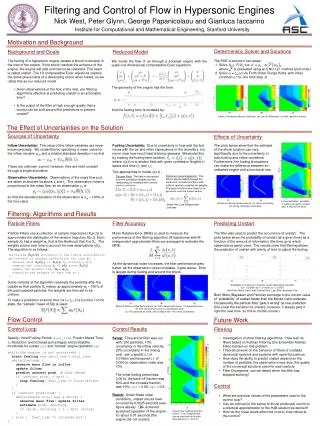
Nick West, Peter Glynn, George Papanicolaou and Gianluca Iaccarino. Institute for Computational and Mathematical Engineering, Stanford University. Motivation and Background. Deterministic Solver and Solutions. Background and Goals. Reduced Model.

E N D
Nick West, Peter Glynn, George Papanicolaou and Gianluca Iaccarino Institute for Computational and Mathematical Engineering, Stanford University Motivation and Background Deterministic Solver and Solutions Background and Goals Reduced Model • The fueling of a hypersonic engine causes a shock to develop in the inlet of the engine. If this shock reaches the entrance of the engine, the engine will stall and cannot be restarted. This event is called unstart. The 1D compressible Euler equations capture the same phenomena of a developing shock when fueled, so we utilize this as our reduced model. • Given observations of the flow in the inlet, are filtering algorithms effective at predicting unstart in an actionable time? • Is the output of the filter of high enough quality that a control can be built around the predictions to prevent unstart? • The PDE is solved in two steps: • Solve Ut = -F(U)xvia: u* = un - t where is evaluated using an ENO-LLF method (2nd order) 2. Solve ut = frhs(u) via Forth Order Runge Kutta, with initial condition u* for one time step t. We model the flow of air through a scramjet engine with the quasi one dimensional compressible Euler equations: The geometry of the engine has the form: And the fueling term is modeled by: (a) (b) (c) Effect of Increasing Mixing Coefficient: (a) Low; (b) Moderate; (c) High, results in unstart. The Effect of Uncertainties on the Solution Filtering and Control of Flow in Hypersonic Engines Sources of Uncertainty Effects of Uncertainty Inflow Uncertainty: The value of the inflow variables are never known precisely. We model this by specifying a mean value for the inflow variable u(i) and a relative standard deviation so that Fueling Uncertainty: Due to uncertainty in how well the fuel mixes with the air and other imprecisions in the chemistry, it is never clear how much heat is being released. We model this by making the fueling term random, where (x,t) is a random field with given correlation lengths in space and time (t and x). The plots below show that the estimate of the shock location can vary significantly due to the uncertainty in both fueling and inflow conditions. Furthermore, the fueling fluctuations can make the difference between an unstarted engine and a functional one. These are unknown a priori, however, they are held constant through a single simulation. Two approaches to model (x,t) : Karhunen Loeve Expansion: The field is approximated through the expansion on basis functions with uniform random variables for weights. The basis functions are taken to be sinusoids over the fueling region. Discrete Field: The field is discretized over the correlation lengths and the randomness is modeled with uniform random variables: Observation Uncertainty: Observations of the mass flow (u) are taken at discrete locations xi and tj. The observation noise is proportional to the mass flow, so an observation yij is so that the standard deviation of the observation is m 100% of the true value. (a) (b) In one realization, variability in fueling can lead to unstart after a second fuel burst. Variance in Shock Location due to: (a) inflow uncertainty; (b) mixing coefficient uncertainty where the I are independent uniforms. Filtering: Algorithms and Results Particle Filters Filter Accuracy Predicting Unstart Particle Filters use a collection of sample trajectories {Xk(x,t)} to approximate the distribution of the random trajectory X(x,t). Each sample Xk has a weight wk that is the likelihood that X is Xk. The weights evolve over time to account for new observations y(tj). The algorithm is as follows: Mean Relative Error (MRE) is used to measure the performance of the filtering algorithm. M trajectories with M independent approximate filters are averaged to estimate the MRE: The filter was used to predict the occurrence of unstart. The plots below show the probability of unstart (at a given time) as a function of the amount of information (the time up to which observations were) used. The results show that filtering allows the prediction of unstart with plenty of time to adjust the fueling. Initialize {Xk(x,0)} according to the inflow distribution while(there is another observation (at time tj)) { advance each Xk(x,tj-1) to Xk(x,tj) by solving a d.e. compute the likelihood lkj of y(tj) given Xk(x,tj) update the weights via: wk wk lkj normalize the weights so they sum to 1 } As the dynamical noise increases, the filter performance gets better; as the observation noise increases, it gets worse. Error is largest during fueling and around the shock. (c) (a) (b) Some variants of the algorithm resample the particles after the update so that particle Xk makes up approximately wk 100% of the post updated particles; the weights are then set to be uniform. Probability of Unstart as a function of last observation included: (a) t = 0.0024; (b) t = 0.0026; (c) t = 0.0027 Dark Blue: Monte Carlo; Red: Particle Filter; Light Blue: Bayesian Filter Both filters (Bayesian and Particle) converge to the correct value of “probability” of unstart faster than the Monte Carlo estimate. Occasionally the particle filter “gets it wrong” at one prediction time (near the transition to unstart), however, it always gets it right the next time, so this is of little concern. To make a prediction at some time tj ≤ t < tj+1 of a function f of the state, the “sample” mean of f(X) is used: (c) (a) (b) Effect of Noise on Filter Performance: (a) 100% observation noise, 1% dynamical noise; (b) 10% observation noise, 1% dynamical noise; (c) 10% observation noise, 30% fueling noise, 10% inflow uncertainty Flow Control Future Work Control Loop Control Results Filtering Specify: Initial Fueling Period: fuel_time, Predict Ahead Time: ∆, Reduction and Increase percentages and probability thresholds for unstart upt and “normal” engine operation spt • Setup:The particle filter was run with: 200 particles; 10% uncertainty in the inflow velocity; 20% uncertainty in the mixing coef. with a spatial c.l. of 0.0166m and temporal c.l. of 0.0001s; observation noise was 10% • The initial fueling period was 0.001s; the back-off fraction was 50% and the increase fraction was 10%; upt = 0.66; spt = 0.9; • Result:Under these initial conditions, unstart should have occurred by 0.0025 seconds (see figure above). We achieved sustained operation of the engine for about 0.01 seconds (the engine did not unstart). • Investigation of other filtering algorithms: How well do filters based on Kalman Filtering (the Ensemble Kalman Filter) behave on this problem. • Theoretical work on the behavior of filters of unstable dynamical systems and systems with rapid fluctuations. • How does the ability to predict unstart depend on the number of particles, the observation noise size, the quality of the numerical solutions used for each particle • Filter Divergence: can we detect when the filter has stopped working? while(the engine is not unstarted) { start fueling now until now + fuel_time while(fueling) { observe mass flow in inflow update filter predict unstart prob. ∆ time ahead if (unstart prob. > upt) { stop fueling; fuel_time *= back-off-pct } } if (unstart predicted) { while(engine still has a shock) { observe mass flow; update filter estimate prob. shocking if (prob. shocking < 1 - spt) {break} } } else { fuel_time *= increase-pct } } Control • What are practical values of the parameters used in the control loop? • Can an optimal (in the sense of thrust produced) control or a practical approximation to the HJB solution be derived? • How do the noise levels effect the control; how robust is the control? Engine flow resulting from the control. The fueling periods can be identified as the dark blue regions in x = [0,0.1].