Download
1 / 35
350 likes | 527 Vues
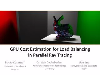
GPU Cost Estimation for Load Balancing in Parallel Ray Tracing. Ugo Erra Università della Basilicata Italy. Carsten Dachsbacher Karlsruhe Institute of Technology Germany. Biagio Cosenza* Universität Innsbruck Austria. Outline. Motivation Parallel Ray Tracing Generating the Cost Map

E N D
GPU Cost Estimation for Load Balancing in Parallel Ray Tracing Ugo ErraUniversità della BasilicataItaly CarstenDachsbacher Karlsruhe Institute of Technology Germany Biagio Cosenza* Universität InnsbruckAustria
Outline • Motivation • Parallel Ray Tracing • Generating the Cost Map • Exploiting the Cost Map for Load Balancing • SAT Adaptive Tiling • SAT Sorting • Results
Ray Tracing Algorithms Toasters, Whitted8.4M primary rays Kalabasha Temple, path tracing134.2M primary rays
Motivation • Load balacing is the major challenge of parallel ray tracing on distributed memory system
Motivation • Load balacing is the major challenge of parallel ray tracing on distributed memory system Ray traced image Cost map
Motivation Can we generate a cost map before rendering? Can we exploit it to improve load balancing? Ray traced image Cost map
Previous work • Ray tracing on distributed memory systems • DSM systems (DeMarle et al. 2005, Ize et al. 2011) • Hybrid CPU/GPU system (Budge et al. 2009) • Massive models (Wald et al. 2004, Dietrich et al. 2007) • Rendering cost evaluation • Profiling (Gillibrand et al. 2006) • Scene geometry decomposition (Reinhard et al. 1998) • Estimate primitive intersections (Mueller et al. 1995)
Parallel Ray Tracing • Image-space parallelization • Scenes that cannot be interactively rendered on a single machine • Target hardware • 1 Master/visualization node (with GPU) • 16 Worker nodes (multi-core CPUs)
ExploitingParallelism in Ray Tracing • Ourapproach • Vectorialparallelism • Intel SSE instruction set (ray packets) • Multi-threading parallelism • pthread • Distributedmemoryparallelism • MPI
ExploitingParallelism in Ray Tracing • Our approach • Vectorial parallelism • Intel SSE instruction set (ray packets) • Multi-threading parallelism • pthread • Distributed memory parallelism • MPI critical for performance!
Our approach • Compute a per-pixel, image-based estimate of the rendering cost, called cost map • Use the cost map for subdivision and/or scheduling in order to balance the load between workers • A dynamic load balancing scheme improves balancing after the initial tiles assignment
Generate the Cost MapImage-space Sampling multiplereflections diffuse specular
Cost Map Generation AlgorithmFor each pixel • Add a basic shader cost for the hit surface • If reflective, compute sampling • Compute the sampling pattern • For each sample, do a visibility check by using the reflection cone • If visible, add the cost of the reflected surface • If the hit surfaces is reflective, add a penalty cost • If the reflection cone of the hit surface hit the first one, add a penalty cost • Gather samples contributions • Use a edge detection filter to raise the cost of “border areas” Ray-packets falling there need to be split and have a higher cost (remarkable only for Whitted)
Sampling Pattern • At first, an uniformly distributed set of points is generated (a) • According to the shading properties, the pattern is scaled (b) and translated to the origin (c) • Lastly, it is transformed according to the projection of the reflection vector in the image plane (d)
Cost Map Results (1) A comparison of the real cost (left) and our GPU-based cost estimate (right)
Limitations and Error Analysis • Off-screen geometry problem (under-estimation due to secondary rays falling out of the screen) • Low sampling rate (under-estimation) • Cost estimation error analysis • (+) Cornell scene: 86% of the predictions fall in the first approximation interval (+/−5% of the real packet time) • (-) Ekklesiasterion scene: 57%
Exploiting the CostMap • Our goal is to improve load balancing • How can we use a cost map estimation for that? • We proposed two approaches • SAT AdaptiveTiling • SAT Sorting
SAT AdaptiveTiling • Adaptive subdivision of the image into tiles ofroughlyequalcost
SAT Adaptive Tiling • We use a Summed Area Table (SAT) for fast cost evaluation of a tile • SAT allows us to compute the sum of values in a rectangular region of an image in constant time • Details in (Crow & Franklin in SIGGRAPH 84) and (Hensley et al. 2005) for the GPU implementation • SAT Adaptive Tiling • Adaptive subdivision of the image • Weighted kd-tree split using the SAT to locate the optimal splits • Details given in the paper
SAT Sorting • Regular (non adaptive) subdivision • Use SAT to sort tasks (=tiles) by estimate • Improve dynamic load balancing • Schedule more expensive tasks at first • Cheaper tiles later • Dynamic load balancing with work stealing • Ensure fine-grained balancing
Dynamic Load Balancingwith Work Stealing • Tile Deque • In-frame steals • Stealing protocol optimizations • Task prefetching master tile assignment workers work stealing
Ray Packet and Tile • Two task definitions • Tile for distributed node • Packet for single node ray tracer • Tile Buffer • Threads work on more tiles • Improved multi threading scalability
ResultsScalability Scalability for up to 16 workers measured for the Cornell Box and path tracing. Timings are in fps.
ResultsWork steal (tile transfers) • Lower number of tile transfers for adaptive tiling • The initial tile assignment provided by the adaptive tiling is more balanced than the regular one • Work stealing does not work well with such kind of (almost balanced) workload Average number of tile transfers performed during our test with 4 workers
Comments • SAT Adaptive Tiling • Needs a very accurate cost map estimate to have an improvement in performance “How much a tile is more expensive than another one?” • Does not fit well with dynamic load balancing • SAT Sorting • It works also with a less accurate Cost Map “Which ones are the more expensive tiles?” • Well fit with the work stealing algorithm • Best performance
Conclusion • Cost map • A per-pixel, image-based estimate of the rendering cost • Cost map exploitation for parallel ray tracing • Two strategies • Cost map generation and exploitation as two decoupled phases • We can mix them with other approaches
Thanks for your attention • Paper’s web pagehttp://www.dps.uibk.ac.at/~cosenza/papers/CostMap • AcknowledgementsFWF, BMWF, DAAD, HPC-Europa2Intel Visual Computing Institute
Cost Map Generation Algorithm • Sampling pattern • Wider sampling pattern for Lambertian and glossy surfaces for path tracing • The pattern collapses to a line for Whitted-style ray tracing and for path tracing using a perfect mirror material. • Sample gathering • By summing up the sample contributions, in path tracing • We suppose that secondary rays spread along a wide area • By taking their maximum, with Whittedray tracing • All samples belong to one secondary ray and we conservatively estimate the cost by taking the maximum. • Edge detection • Ray-packet splitting raises the cost because of the loss of coherence between rays, and this happens especially in “geometric edges” • We experienced that this extra cost is significant only with Whitted ray tracing • Implementation uses deferred shading, with a 2nd sampling pass
Cost Map Generation Algorithm Code for pixel Pi • //All the data of the hit surface on the pixel Pi are available • costi ← basic material cost of the hit surface; • if Pi is reflective then • //Determinate the sampling pattern S, at the point Pi, toward the reflection vector R • S = compute_sampling_pattern(Pi,R); • // For each samples, calculate cost contribute • for each sample S j in S do • sample j ← 0; • ifvisibility_check(Sj,Pi) then • increase samplej; • if secondary reflection check(Sj,Pi) then • increase samplej; • end • end • end • //Samples gathering • costi = costi + gather(S); • end • return costi;
Error Analysis Error distribution of the estimation. Each packet-based rendering time is subtract from the cost map estimate, for the same corresponding packet of pixels. The x-axis shows the difference in error intervals, from negative values (left, over-estimation) to positive ones (right, under-estimation). The y-axis plots error occurrences for each error interval.