Download
1 / 16
160 likes | 442 Vues
The semi-Lagrangian technique. x. x. x. x. x. x. x. x. x. The semi-Lagrangian technique. material time derivative or time evolution along a trajectory. no quadratic terms. x. From a regular array of points we end up after Δ t with a non-regular distribution. x. x. x. x.

E N D
x x x x x x x x x The semi-Lagrangian technique material time derivative or time evolution along a trajectory no quadratic terms x From a regular array of points we end up after Δt with a non-regular distribution x x x x x x x x Semi-Lagrangian: tracking back Solution of the one-dimensional advection equation: origin point computing the origin point
Linear advection equation without r.h.s. Stability in one dimension p Origin of parcel at j: X*=Xj-U0Δt x j multiply upstream α p: integer Linear interpolation α is not the CFL number except when p=0, then=> upwind Von Neumann: |λ|≤1 if 0 ≤α≤1 (interpolation from two nearest points) damping
Cubic spline interpolation S(x) is a cubic polynomial - S(xj)=φj at the neighbouring grid points - ∂S(x)/ ∂x is continuous - ∫d2S/dx2 dx is minimal Then: S(x)=Dj-1(xj-x)2(x-xj-1)/(Δx)2-Dj(x-xj-1)2(xj-x) /(Δx)2 + +φj-1(xj-x)2[2(x-xj-1)+ Δx] /(Δx)3+ φj(x-xj-1)2[2(xj-x)+ Δx] /(Δx)3 where (Dj-1+4Dj+Dj+1)/6=(φj+1- φj-1)/2 Δx
Cubic Lagrange interpolation Q(x) is a cubic polynomial - Q(xj)= φj at 4 nearest grid-points
x x x x x x Shape-preserving interpolation • Creation of artificial maxima /minima x: grid points x x x x: interpolation point x x • Shape-preserving and quasi-monotone interpolation - Spline or Hermite interpolation derivatives modified derivatives interpolation - Quasi-monotone interpolation x φmax x φmin
o o x x 3-t-l Semi-Lagrangian schemes in 2-D L: linear operatorN: non-linear function • Interpolating G x x x x x x x x x x x x I x Two interpolations needed • Ritchie scheme U=U*+U’ V=V*+V’ G x x x x x x x x x x x x I’ 2V*Δt o’ 2V’Δt • Non-interpolating Average the non-linear terms between points G and o’ The three of them are second-order accurate in space-time
Bicubic: underlined points Details about interpolation 12-point interpolation in 2-D; 32-point interpolation in 3-D: red points Bilinear: shadowed points x x x x x xxxx x xxxx x xxxx x xxxx x G x o
Stability of 2-D schemes • In the linear advection equation the interpolating scheme is stable provided the interpolations use the nearest points • In the linear shallow-water equations, treating the linear terms implicitly, the stability limit is • In the two non-interpolating schemes the stability is given by • Advective treatment of Coriolis term Δt f ≤1 Coriolis term (kU’+lV’) Δt ≤1 Which is always true due to the definition of U’ and V’
Spherical geometry in semi-Lagrangian advection Z V x G j j j Y i G X O I i i Trajectory calculation Tangent plane projection
V1Δt Iterative trajectory calculation V0Δt x x x x x x x x x x x x x x x x x x x x x x x x x r0 r1 can be taken as trajectory straight line or great circle or as implicit assumed constant during 2Δt
Iterative trajectory computation (1 dimension) rn+1=g-VnΔt Where, for simplicity, we have taken a 2-time-level scheme and taken the velocity at the departure point of the trajectory Assume that V varies linearly between grid-points V=a+b.rb=dV/dr (divergence) r n+1 = g - aΔt - Δt b rn For this procedure to converge, it must have a solution of the form r = λn + K; (| λ| < 1) Substituting, we get K=(g - a Δt)/(1 + b Δt) and λ = -b Δt therefore we must have The condition means thet the parcels do not overtake eachother is less restrictive than the CFL condition, in general doesn’t depend on the mesh size
Semi-Lagrangian equation with right-hand-side • Three-time-level schemes - centered (second-order accurate) scheme the r.h.s. R can be evaluated by interpolation to the middle of the trajectory or averaged along the trajectory: RM(t)={RD(t)+RA(t)}/2 - split in time (first-order accurate) - R at the departure point (first-order accurate)
Example Let us apply each of the above schemes to the equation whose analytical solution (with appropriate initial and boundary conditions) is: Z = Re( Ae-ikx eωt) with ω=ikU0-k2K WARNING: the three-time-level scheme applied to the diffusion eq. has an absolutely unstable numerical solution With the values A=1, k=2π/100, K=10-2, the r.m.s. error with respect to the analytical solution (before the unstable numerical solution grows too much) grows linearly with time. After 200 sec of integration, the error is: 5×10⁻⁴Δt for the split treatment 5×10⁻⁴Δt for r.h.s. at departure point 5×10⁻⁸ (Δt)2 for the centered scheme
Semi-Lagrangian equation with right-hand-side (cont) • Two-time-level schemes - centered scheme with - split or R at the departure point similar to the 3-time-level case - SETTLS scheme Taylor expansion around the departure point and
Trajectory computation with SETTLS Mean velocity during Δt The Taylor expansion from which we started is: which represents a uniformly accelerated movement The middle of the trajectory is not the average between the departure and the arrival points