Download
1 / 33
350 likes | 439 Vues
Review of statistical modeling and probability theory. Alan Moses ML4bio. What is modeling?. Describe some observations in a simple, more compact way. X = (X 1 ,X 2 ). What is modeling?. Describe some observations in a simple, more compact way. G m. Model: a = -. r 2.

E N D
Review of statistical modeling and probability theory Alan Moses ML4bio
What is modeling? • Describe some observations in a simple, more compact way X = (X1,X2)
What is modeling? • Describe some observations in a simple, more compact way G m Model: a = - r2 Instead of all the observations, we only need to remember a constant ‘G’ and measure some parameters ‘m’ and ‘r’.
What is statistical modeling? • Deals also with the ‘uncertainty’ in observations Deviation or Variance Expectation • Mathematics is more complicated • Also use the term ‘probabilistic’ modeling
What kind of questions will we answer in this course? What’s the best linear model to explain some data?
What kind of questions will we answer in this course? Are there multiple groups? What are they?
What kind of questions will we answer in this course? Given new data, which group do we assign it to?
3 major areas of machine learning (that have proven useful in biology) • Regression • Clustering • Classification
Molecular Biology example X = (L,D) Expression Level Expectation Variance disease
Molecular Biology example “clustering” V1 E1 Expression Level Expression Level Expectation Variance Class 2 is “enriched” for disease E2 V2 disease
Molecular Biology example “clustering” V1 E1 Expression Level Expression Level Expectation Variance Class 2 is “enriched” for disease E2 V2 disease “regression” Expression Level AA Aa aa Genotype
Molecular Biology example “clustering” V1 E1 Expression Level Expression Level Expectation Variance Class 2 is “enriched” for disease E2 V2 disease “classification” “regression” Expression Level Expression Level Aa disease? AA Aa aa AA Aa aa Genotype Genotype
Probability theory • Probability theory quantifies uncertainty using ‘distributions’ • Distributions are the ‘models’ and they depend on constants and parameters E.g., in one dimension, the Gaussian or Normal distribution depends on two constants e and π and two parameters that have to be measured, μ and σ (X–μ)2 – e 2σ2 1 P(X|μ,σ) = √2πσ2 ‘X’ are the possible datapoints that could come from the distribution. In statistics jargon ‘X’ is called a random variable
Probability theory • Probability theory quantifies uncertainty using ‘distributions’ • Choosing the distribution or ‘model’s the first step in a statistical model • E.g., data: mRNA expression levels, counts of sequencing reads, presence or absence of protein domains or ‘A’ ‘C’ ‘G’ and ‘T’ s • We will use different distributions to describe these different types of data.
Typical data and distributions • Data is categorical (yes or no, A,C,G,T) • Data is a fraction (e.g., 13 out of 5212) • Data is a continuous number (e.g., -6.73) • Data is a ‘natural’ number (0,1,2,3,4…) • It’s also possible to do regression, clustering and classification without specifying a distribution
Molecular Biology example • In this example, we might try to combine a Bernoulli for the disease data, Poisson for the genotype and Gaussian for the expression level • We also might try to classify without specifying distributions “classification” Expression Level Aa disease? AA Aa aa Genotype
Molecular Biology example • genomics era means we will almost never have the expression level for just one gene or the genotype at just one locus • Each gene’s expression level can be considered another ‘dimension’ • for two genes, if each point is data for one person, we can make a graph of this type of data • for 1000s of genes…. Gene 3 Gene 4 Gene 2 Expression Level Gene 2 Expression Level Gene 5 … Gene 1 Expression Level Gene 1 Expression Level
Molecular Biology example • genomics era means we will almost never have the expression level for just one gene or the genotype at just one locus • We’ll usually make 2-D plots, but anything we say about 2-D can usually be generalized to n-dimensions Each “observation” , X, contains expression level for Gene 1 and Gene 2 Represent this as a vector: Gene 2 Expression Level X = (1.3, 4.6) e.g., X = (X1, X2) Or generally Gene 1 Expression Level
Molecular Biology example • genomics era means we will almost never have the expression level for just one gene or the genotype at just one locus • We’ll usually make 2-D plots, but anything we say about 2-D can usually be generalized to n-dimensions Each “observation” , X, contains expression level for Gene 1 and Gene 2 Represent this as a vector: Gene 2 Expression Level X = (1.3, 4.6) e.g., X = (X1, X2) Or generally This gives a geometric interpretation to multivariate statistics Gene 1 Expression Level
Probability theory • Probability theory quantifies uncertainty using ‘distributions’ • Distributions are the ‘models’ and they depend on constants and parameters E.g., in two dimensions, the Gaussian or Normal distribution depends on two constants e and π and 5 parametersthat have to be measured, μ and Σ (X–μ)T Σ-1 (X–μ) 1 – e 2 1 What does the mean mean in 2 dimensions? What does the standard deviation mean? P(X|μ,σ) = 2π √|Σ| ‘X’ are the possible datapoints that could come from the distribution. In statistics jargon ‘X’ is called a random variable
Molecular Biology example • genomics era means we will almost never have the expression level for just one gene or the genotype at just one locus • We’ll usually make 2-D plots, but anything we say about 2-D can usually be generalized to n-dimensions Each “observation” , X, contains expression level for Gene 1 and Gene 2 X = (X1, X2) Represent this as a vector: µ µ = (µ1, µ2) Gene 2 Expression Level The mean is also a vector: σ12 σ11 Σ = The variance is a matrix: σ21 σ22 Gene 1 Expression Level
µ Σ = Σ = 1 0 0 1 1.0 0.5 0.5 1.0 “spherical covariance” “correlated data” Σ = σ2I Σ = 1 0 0 4 Σ = 1.0 -1.9 -1.9 4.0 “axis-aligned, diagonal covariance” “full covariance”
Probability theory • Probability theory quantifies uncertainty using ‘distributions’ • Distributions are the ‘models’ and they depend on constants and parameters • Once we chose a distribution, the next step is to chose the parameters • This is called “estimation” or “inference” (X–μ)2 – e 2σ2 1 P(X|μ,σ) = √2πσ2
Estimation • We want to make a statistical model. • Choose a model (or probability distribution) • Estimate its parameters Expression Level Expectation Variance • Choose the parameters so the model ‘fits the data’ • There are many ways to measure how well a model fits that data • Different “Objective functions” will produce different “estimators” (E.g., MSE, ML, MAP) (X–μ)2 – e 2σ2 1 P(X|μ,σ) = √2πσ2 How do we know which parameters fit the data?
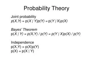
Laws of probability (True for all distributions) • If X1 … XN are a series of random variables (think datapoints) P(X1 , X2) is the “joint probability” and is equal to P(X1) P(X2) if X1 and X2 are independent. P(X1 | X2), is the “conditional probability” of event X1given X2 Conditional probabilities are related by Bayes’ theorem: P(X1) P(X1| X2) = P(X2 |X1) P(X2)
Likelihood and MLEs • Likelihood is the probability of the data (say X) given certain parameters (say θ) • Maximum likelihood estimation says: choose θ, so that the data is most probable. • In practice there are many ways to maximize the likelihood. L = P(X|θ) L = 0 θ
Example of ML estimation Data: Xi P(Xi|μ=6.5, σ=1.5) L = P(X|θ) = P(X1 … XN | μ, σ) 5.2 9.1 8.2 7.3 7.8 0.182737304 0.059227322 0.13996368 0.230761096 0.182737304 i=5 Π = P(Xi|μ=6.5, σ=1.5) = 6.39 x 10⁻⁵ i=1 L Mean, μ
Example of ML estimation In practice, we almost always use the log likelihood, which becomes a very large negative number when there is a lot of data Mean, μ Log(L)
Example of ML estimation Log(L) Standard deviation, σ Mean, μ
ML Estimation • In general, the likelihood is a function of multiple variables, so the derivatives with respect to all of these should be zero at a maximum • In the example of the Gaussian, we have two parameters, so that • In general, finding MLEs means solving a set of coupled equations, which usually have to be solved numerically for complex models. L = 0 L = 0 and μ σ
MLEs for the Gaussian 1 1 Σ Σ • The Gaussian is the symmetric continuous distribution that has as its “centre” a parameter given by what we consider the “average” (the expectation). • The MLE for the for variance of the Gaussian is like the squared error from the mean, but is actually a biased (but still consistent!?) estimator μML = X VML = (X - μML)2 N N X X
Other estimators • Instead of likelihood, L = P(X|θ) we can choose parameters to maximize posterior probability: • Or sum of squared errors: • Or a penalized likelihood: L* = P(X|θ) • In each case, estimation involves a mathematical optimization problem that usually has to be solved on computer • How do we choose? P(θ|X) Σ (X – μMSE)2 X – θ2 e x