Download
1 / 68
710 likes | 1.42k Vues
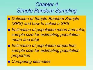
Chapter 4 Simple Random Sampling. Random Samples and Simple Random Samples (SRS) and how to select a SRS Estimation of population mean and total; sample size for estimating population mean and total Estimation of population proportion; sample size for estimating population proportion

E N D
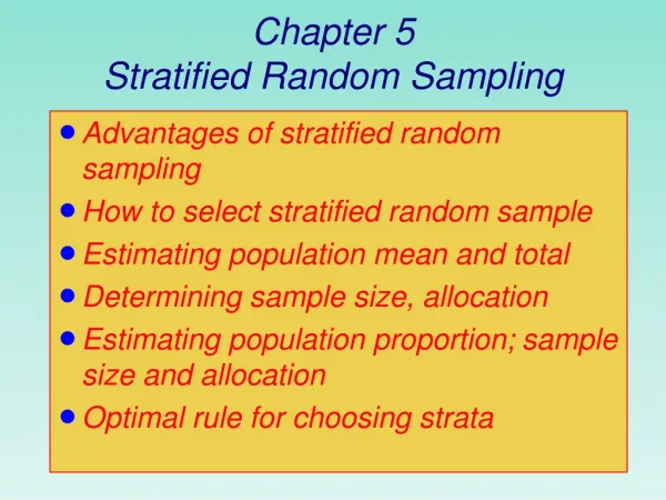
Chapter 4Simple Random Sampling • Random Samples and Simple Random Samples (SRS) and how to select a SRS • Estimation of population mean and total; sample size for estimating population mean and total • Estimation of population proportion; sample size for estimating population proportion • Comparing estimates
Random Samples • Desire the sample to be representative of the population from which the sample is selected • We use RandomSamples: each element in the population has an equal chance to be selected.
Example: Random Sample • Suppose a large Statistics class of 500 students has 250 male and 250 female students. • To obtain student feedback about the course, I select 250 students from the class by flipping a fair coin one time. • If the coin shows heads, I select the 250 males as my sample; if the coin shows tails I select the 250 females as my sample. • What is the chance any individual student from the class is included in the sample? 1/2 Every sample consists of only 1 gender – hardly representative. Yes! Is this a random sample? Is this random sample a representative sample from the class? No!
Simple Random Sample RandomSample: each element in the population has an equal chance to be selected. • A simple random sample (SRS) of size n consists of n units from the population chosen in such a way that every possible group of n unitshas an equal chanceto be the sample actually selected. SIMPLE random sampling (start at 2:10) Simple random sampling takes random sampling1 step further
Simple Random Samples (cont.) • The easiest way to choose an SRS is with random numbers. Statistical software cangenerate random digits (e.g., Excel “=random()”, ran# button on calculator).
Example: simple random sample • The Statistics Club wishes to randomly choose a 3-member committee from the 28 members of the club. 00 Abbott 07 Goodwin 14 Pillotte 21 Theobald 01 Cicirelli 08 Haglund 15 Raman 22 Vader 02 Crane 09 Johnson 16 Reimann 23 Wang 03 Dunsmore 10 Keegan 17 Rodriguez 24 Wieczoreck 04 Engle 11 Lechtenb’g 18 Rowe 25 Williams 05 Fitzpat’k 12 Martinez 19 Sommers 26 Wilson 06 Garcia 13 Nguyen 20 Stone 27 Zink
Solution • Use a random number table; read 2-digit pairs until you have chosen 3 committee members • For example, start in row 121: • 71487 09984 29077 14863 61683 47052 62224 51025 Garcia (07) Theobald (22) Johnson (10) • Your calculator generates random numbers; you can also generate random numbers using Excel
Sampling Variability • Suppose we had started in line 145? • 19687 12633 57857 95806 09931 02150 43163 58636 • Our sample would have been 19 Rowe, 26 Williams, 06 Fitzpatrick
Sampling Variability • Samples drawn at random generally differ from one another. • Each draw of random numbers selects different people for our sample. • These differences lead to different values for the variables we measure. • We call these sample-to-sample differences sampling variability. • Variability is OK; bias is bad!!
Example: simple random sample • Using Excel tools • Using statcrunch (NFL)
4.3 Estimation of population mean µ • Usual estimator
4.3 Estimation of population mean µ • For a simple random sample of size n chosen without replacement from a population of size N • The correction factor takes into account that an estimate based on a sample of n=10 from a population of N=20 items contains more information than a sample of n=10 from a population of N=20,000
4.3 Estimating the variance of the sample mean • Recall the sample variance
4.3 Example • Population {1, 2, 3, 4}; n = 2, equal weights
4.3 Example • Population {1, 2, 3, 4}; µ=2.5, σ2 = 5/4; n = 2, equal weights
4.3 Example • Population {1, 2, 3, 4}; µ=2.5, σ2 = 5/4; n = 2, equal weights
4.3 Example Summary • Population {1, 2, 3, 4}; µ=2.5, σ2 = 5/4; n = 2, equal weights
t distributions • Very similar to z~N(0, 1) • Sometimes called Student’s t distribution; Gossett, brewery employee • Properties: i) symmetric around 0 (like z) ii) degrees of freedom
Student’s t Distribution P(t > 2.2281) = .025 P(t < -2.2281) = .025 .95 .025 .025 t10 0 -2.2281 2.2281
Standard normal P(z > 1.96) = .025 P(z < -1.96) = .025 .95 .025 .025 z 0 -1.96 1.96
Z t -3 -2 -1 0 1 2 3 -3 -2 -1 0 1 2 3 Student’s t Distribution Figure 11.3, Page 372
Degrees of Freedom Z t1 -3 -2 -1 0 1 2 3 -3 -2 -1 0 1 2 3 Student’s t Distribution Figure 11.3, Page 372
Degrees of Freedom Z t1 t7 -3 -2 -1 0 1 2 3 -3 -2 -1 0 1 2 3 Student’s t Distribution Figure 11.3, Page 372
4.3 Margin of error when estimating the population mean µ • Understanding confidence intervals; behavior of confidence intervals.
Comparing t and z Critical Values Conf. level n = 30 z = 1.645 90% t = 1.6991 z = 1.96 95% t = 2.0452 z = 2.33 98% t = 2.4620 z = 2.58 99% t = 2.7564
Required Sample Size To Estimate a Population Mean • If you desire a C% confidence interval for a population mean with an accuracy specified by you, how large does the sample size need to be? • We will denote the accuracy by MOE, which stands for Margin of Error.
Example: Sample Size to Estimate a PopulationMean • Suppose we want to estimate the unknown mean height of male students at NC State with a confidence interval. • We want to be 95% confident that our estimate is within .5 inch of • How large does our sample size need to be?
Good news: we have an equation • Bad news: • Need to know s • We don’t know n so we don’t know the degrees of freedom to find t*n-1
Confidence level Sampling distribution of y .95
Estimating s • Previously collected data or prior knowledge of the population • If the population is normal or near-normal, then s can be conservatively estimated by s range 6 • 99.7% of obs. Within 3 of the mean
Example:samplesize to estimate mean height µ of NCSU undergrad. male students We want to be 95% confident that we are within .5 inch of , so • MOE = .5; z*=1.96 • Suppose previous data indicates that s is about 2 inches. • n= [(1.96)(2)/(.5)]2 = 61.47 • We should sample 62 male students
Example: Sample Size to Estimate a PopulationMean -Textbooks • Suppose the financial aid office wants to estimate the mean NCSU semester textbook cost within MOE=$25 with 98% confidence. How many students should be sampled? Previous data shows is about $85.
Example: Sample Size to Estimate a Population Mean -NFL footballs • The manufacturer of NFL footballs uses a machine to inflate new footballs • The mean inflation pressure is 13.0 psi, but random factors cause the final inflation pressure of individual footballs to vary from 12.8 psi to 13.2 psi • After throwing several interceptions in a game, Tom Brady complains that the balls are not properly inflated. The manufacturer wishes to estimate the mean inflation pressure to within .025 psi with a 99% confidence interval. How many footballs should be sampled?
Example: Sample Size to Estimate a Population Mean • The manufacturer wishes to estimate the mean inflation pressure to within .025 pound with a 99% confidence interval. How may footballs should be sampled? • 99% confidence z* = 2.58; ME = .025 • = ? Inflation pressures range from 12.8 to 13.2 psi • So range =13.2 – 12.8 = .4; range/6 = .4/6 = .067 . . . 1 2 3 48
Required Sample Size To Estimate a Population Mean • It is frequently the case that we are sampling without replacement.
Required Sample Size To Estimate a Population Mean When Sampling Without Replacement.
Required Sample Size To Estimate a Population Mean When Sampling Without Replacement.
Required Sample Size To Estimate a Population Mean When Sampling Without Replacement.
4.3 Estimation of population total • Estimate number of lakes in Minnesota, the “Land of 10,000 Lakes”.