Download
1 / 54
570 likes | 701 Vues
Machine Learning Introduction. Why is machine learning important? AI systems are brittle, learning can improve a system’s capabilities AI systems require knowledge acquisition, learning can reduce this effort

E N D
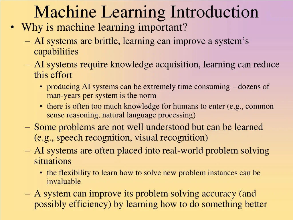
Machine Learning Introduction • Why is machine learning important? • AI systems are brittle, learning can improve a system’s capabilities • AI systems require knowledge acquisition, learning can reduce this effort • producing AI systems can be extremely time consuming – dozens of man-years per system is the norm • there is often too much knowledge for humans to enter (e.g., common sense reasoning, natural language processing) • Some problems are not well understood but can be learned (e.g., speech recognition, visual recognition) • AI systems are often placed into real-world problem solving situations • the flexibility to learn how to solve new problem instances can be invaluable • A system can improve its problem solving accuracy (and possibly efficiency) by learning how to do something better
How Does Machine Learning Work? • Learning in general breaks down into one of a few forms • Learning something new • no prior knowledge of the domain/concept • no previous representation • we need to add new information to the knowledge base • Learning something new about something you already know • add to the existing knowledge base or refine the knowledge base • modification of the previous representations • Learning how to do something better, either more efficiently or with more accuracy • previous problem solving instance (case, chain of logic) can be “chunked” into a new rule (also called memoizing) • previous knowledge can be modified – typically this is a parameter adjustment like a weight or probability in a network that indicates that this was more or less important than previously thought
Types of Machine Learning • There are many ways to implement ML • Supervised vs. Unsupervised (discovery) vs. Reinforced • is there a “teacher” that rewards/punishes right/wrong answers? • Symbolic vs. Subsymbolic vs. Evolutionary • at what level is the representation? • subsymbolic is the fancy name for neural networks • evolutionary learning is actually a subtype of symbolic learning • Knowledge acquisition vs. Learning through problem solving vs. Explanation-based learning vs. Analogy • We can also focus on what is being learned • Learning functions • Learning rules • Parameter adjustment • Learning classifications • these are not mutually exclusive, for instance learning classification is often done by parameter adjustment or by learning a function
The idea behind supervised learning is that the learning system is offered examples The system uses what it already knows to respond to an input if correct, system strengthens components that led to the right answer if incorrect, system weakens components that led to the wrong answer This is performed for each item in the training set Repeat some number of iterations or until the system “converges” to an answer Once “trained”, we test the system with the testing set data Note that supervised learning can result in an “overtrained” structure so that it learns the training set but does not translate well to the testing set Supervised Learning
Continued • Supervised learning is actually a search problem • Search for the representation that will allow it to respond correctly to every (or most) instance in the training set • there could be many “correct” solutions • some of these will also allow the system to respond correctly to most instances in the testing set
Unsupervised Learning • Here, we present unlabeled data to the system • It attempts to find hidden patterns within the data • This is an attempt at knowledge discovery • Data mining is a form of unsupervised learning (e.g.,clustering, rule induction) • Statistical methods are commonly used to find similarities and differences among the data to segregate the data into meaningful classes or groupings • For a hidden Markov model, the E-M (or Baum Welch) algorithm to learn or improve its probabilities is a form of unsupervised learning • In neural networks, the self-organizing map is a form of unsupervised learning
Reinforcement Learning • A form of learning through trial and error where feedback is not a correct answer (as with supervised learning) but a utility or feedback function • This function does not tell us if we have a right answer but instead evaluates the answer in terms of how useful it is • We would like to maximize utility • One example is to minimize the effort needed to achieve the output, so our reinforcement utility function determines effort and attempts to modify the process so that the next time we reach this output state, we have done so with less effort • Implementations include • Genetic algorithms where the utility function is our fitness function • Statistical search approaches using dynamic programming along with a utility function to evaluate each path • Neural networks
Types of Learning • We will explore several different forms of learning in this and the next lecture • We can view learning as one of • classification – training data mapped to a class • regression – training data mapped to continuous values/function • Or, we can view learning based on the specific algorithmic approach • Inductive learning (supervised) • Support vector machines* (supervised) • Discovery/similarity learning (unsupervised) • Reinforcement learning (utility function)** • Probabilistic (unsupervised or reinforcement) • Explanation-based learning*** • * - covered next week, ** - covered minimally next week, • *** - not covered
Learning Within a Concept Space • A concept space consists of the features used to represent a particular class • our task is to learn the proper values for the features that describe legal entities in the class • By introducing positive and negative examples, we learn the class – this is called inductive learning • instances are hits and misses • working one example at a time, we represent the class by legal values for each feature • generalizing the representation for positive instances • specializing the representation for negative instances
Candidate Elimination • One approach is through candidate elimination • G is the set of values that represent our current general description • S is the set of values that represent our most specific description • process iterates over + and - examples • specialize G with - ex • generalize S with + ex • until the two representations are equal • or until they become empty, in which case the examples do not lead to a single representation for the given class
Discovery • We have data and want to learn something from it • Unsupervised – we do not know what the data might tell us • Primarily use statistical methods to explore data • Data might not be set up for data mining so we have to modify the data first • change values in a continuous range into discrete values (e.g., converting age to a class such as “child”, “teen”, “adult”, “senior” • we might need to anonymize the data for privacy concerns • we might have to remove certain fields that may not be useful – for instance, address may not be relevant for medical data discovery • We explore three data mining approaches here
The basic idea behind the decision tree dates back to the 1960s as a form of automated induction (updated in the 1970s by Quinlan and the ID3 algorithm) Use training data to generate a tree that divides the training data into decision classes where branches of the tree are based on values of a selected feature (e.g., one branch for age < 20, one for age >= 20) Given a set of data, create a tree that will predict what a new datum will be categorized as Decision trees are sometimes referred to as classification trees, regression trees (when the output is not a class but instead a real value) or CART, based on a newer algorithm that produces multiple trees in order to find the best decision tree Decision Trees
Decision Tree Algorithms • The basic algorithm works as follows: • Given all data, find the attribute that divides the data set most cleanly into categories/classes/decisions (e.g., the “play golf” and the “do not play golf” categories) • what does it mean to most cleanly divide into categories? • this measure of dividing data into sets is known as information gain and is based on the statistical principle of entropy • Create a node in the tree that represents this attribute and create one edge leaving this node for each possible attribute value • Recursively do the same at each successive branch • Stop recursing when • all data fall into one category, or • there are no more attributes to apply, or • you have reached a threshold value such as a maximum tree depth or a minimum number of elements left in the data set for this given node
Information Gain and Entropy • Entropy tells you how likely the given feature will lead to a proper classification • by computing the entropy of the entire group, you can maximize information gain by selecting the feature which leads to a minimum entropy • Information gain itself is a distance from an estimated probability to an actual probability • information gain can be interpreted as the expected extra message-length per datum that must be communicated if a code that is optimal for a given (wrong) distribution Q is used, compared to using a code based on the true distribution P • where nb = number of instances in branch b, nbc = number of instances of class c in branch b, nt= total number of all instances in all branches
Clustering • Given data with n features, map these in n-dimensional space • Identify groups that are “near” to each other • we usually compute the distance between data using a Euclidian distance-like formula • D = ((x11 – x21)2 + (x12 – x22)2 + … + (x1n – x2n)2)1/2 • this approach might tell us what data cluster together but not why the cluster exists or what the cluster represents • it is usually up to humans to then explore each cluster and perhaps identify its significance or name • In k-means clustering, we select k data to represent the centers of clusters and then for each new datum, determine which cluster center it is closest to and thus build clusters in this way • Once generated, we repeatedly perform this task using the cluster centers so that we do not bias our clusters by the first k data selected
Some clusters will reflect classes of interest, others may be artifacts of data or algorithm One way to attempt to ensure useful clusters is to create the clusters hierarchically create small clusters add data to clusters combine similar clusters until either all data belong to a cluster or some threshold has been passed Two techniques: divisive (top down) – start with one big set and begin to divide into 2 or more classes by using some distinguishing feature agglomerative (bottom up) – group data together into a class, and then group classes together, … Hierarchical Clustering
Fuzzy Clustering • Recall in fuzzy set theory, an element exists in every set to some extent • In fuzzy clustering, a datum belongs to every cluster to some extent, that extent is determined through fuzzy calculations • this allows data that are on the edge of several clusters to be in multiple clusters • we define the membership value as uk(x) which provides a real number [0, 1] of how well x fits into cluster k and where the sum of all ui(x) for all i will be 1.0 • we define the center of a cluster to be: • and then • A learning algorithm, much like that of k-means, is used to create initial clusters and then identify fuzzy clustering for test data
Ensemble of Classifiers • Clustering algorithms and decision trees produce/represent classifiers • A classifier will only be as good as the training data • and even then, classifiers may be over or under trained • We can instead generate multiple classifiers from the same training data • each classifier might be trained on different data, different subsets of data or different features of the data, or by different algorithms • this may help prevent training bias from impacting the performance of our classifiers • Now we use the ensemble for classification by using some voting scheme • simple majority rule vote • a weighted vote • a vote using scoring from each classifier (add up the strengths of their beliefs)
A generic form of ensemble learning is called Boosting produce an ensemble classifier which might include poorly trained classifiers and then learn under which conditions which classifiers are more trustworthy the AdaBoost algorithm is shown to the below here, we are training a set of classifiers H consisting of individual classifiers Dt(i) (classifier i at time t) and using at as a training factor specialized to that classifier and that input Boosting • We train our classifiers • And then we iteratively determine when each classifier is inaccurate and reduce its relative weighting in the overall decision making for the given class
Rule Induction • An easily obtained set of information is association rules which are derived by finding patterns in the data through counting appearances • In n of m records, features Y and Z both occur • If n / m > threshold, we might consider Y and Z to be related through association • The common usage is to identify common trends • Of 1000 store receipts, 700 customers bought bread and of those 700, 500 bought milk • Therefore we consider bread and milk to be related • We might then move the bread and milk closer together or offer a deal that if you buy bread you get milk ¼ off • Unfortunately, rule induction may provide rules without any kind of meaning since it merely finds associations
Measuring Rules • 3 measurables are: • Accuracy – how often is the rule correct? Count(A & B) / Count(A) • Coverage – how often does the rule apply? Count(A) / All records examined • Interestingness – how interesting is this rule? A relative term computed by combining accuracy and coverage • Example: store statistics show for 100 shopping baskets • number with eggs = 30, number with milk 40, number with cheese = 10, number with both eggs and milk 20, number with both eggs and cheese = 5 • Rule1: People who buy milk will buy eggs, accuracy = 20 / 40 = 50%, coverage = 20 / 100 = 20%, • Rule2: People who buy eggs will buy cheese, accuracy = 5 / 30 = 17%, coverage = 5 / 100 = 5% • Rule 1 is more interesting, having both greater accuracy and coverage
Probabilistic Learning • Naïve Bayes classifiers, Bayesian nets and hidden Markov models all require probabilities • We can “learn” probabilities through counting • p(a) = number of occurrences of a out of all data • p(a | b) = number of occurrences of a when b is true • we can obtain these directly from a data set • we need to make sure the data set is not biased or our probabilities may not be very accurate • Two forms of learning for Bayesian nets and HMMs are • Learning the structure of the network from data (this is more commonly applied to Bayesian nets) • Learning parameters (probabilities) by applying data to the network/HMM and then modifying these parameters to improve the accuracy – we will use the E-M (Emission, Modification) algorithm
Naïve Bayesian Learning • We want to learn, given some conditions, whether to play tennis or not • see the table on the next page • The data available generated tells us from previous occurrences what the conditions were and whether we played tennis or not during those conditions • there are 14 previous days’ worth of data • To compute our prior probabilities, we just do • P(tennis) = days we played tennis / totals days = 9 / 14 • P(!tennis) = days we didn’t play tennis = 5 / 14 • The evidential probabilities are computed by adding up the number of Tennis = yes and Tennis = no for that evidence, for instance • P(wind = strong | tennis) = 3 / 9 = .33 and P(wind = strong | !tennis) = 3 / 5 = .60
Continued • We do not have enough data for some combinations of conditions leading to probabilities of 0 • we do not want to use 0% probabilities so we will add an absolute minimum probability to apply in such cases • We must rely on the Naïve Bayesian assumption of conditional independence to get around this problem P(Sunny & Hot & Weak | Yes) = P(Sunny | Yes) * P(Hot | Yes) * P(Weak | Yes)
Learning Structure • For a Bayesian network, how do we know what states should exist in our structure? How do we know what links should exist between states? • There are two forms of learning here • to learn the states that should exist • to learn which transitions should exist between states • States are the variables found in the data (unless we build junction trees) so is not particularly interesting to learn • Two algorithms to learn transitions are • Score and search – generate a BN from the data, generate “neighbor” BNs (those that you can obtain by adding or removing edges) and evaluate them, retain the best BN and repeat • Constraint-based – edges represent dependencies, learn these by evaluating the data
Example • Given a collection of research articles, learn the structure of a paper’s header • that is, the fields that go into a paper • Data came in three forms: labeled (by human), unlabeled, distantly labeled (data came from bibtex entries, which contains all of the relevant data but had extra fields that were to be discarded) from approximately 5700 papers • the transition probabilities were learned by simple counting
HMMs • Recall the Markov model combined a network of nodes in which we had prior probabilities and transition probabilities • Most interesting AI problems cannot be solved by a Markov model because there are unknown states in our real world problems • we see the effects of some cause but want to know what the cause is • A hidden Markov model (HMM) is a Markov model which includes hidden nodes and an additional form of probability – emission probability • that is, the probability that the effect of the node would arise given that the cause is true • now, to compute a cause, we find the most probable path through the Markov model where the probability of the path is the product of the prior probability of each node, the transition probability between each node, and the emission probability that the node would occur given a hidden node
More • HMMs often consist of just a few states repeated to represent a change in time to represent a likely sequence • There are 3 problems that HMMs can be used to solve • Given an HMM, compute the probability of a given output sequence – this is not AI but might be used for prediction • Given an HMM and an output sequence, compute the most likely state transitions – here, we are trying to determine the most likely cause of the events witnessed (diagnosis, speech recognition, etc) • Given an HMM and an output sequence, learn (or tune) the probabilities that make up the HMM
HMM Problem 1 • Problem 1: given an HMM and an output sequence, compute the probability of generating that particular output sequence (e.g., what is the likelihood of seeing this particular sequence of observations?) • We have an observation sequence O: O1 O2 O3 … Ok and states • Recall that we have 3 types of probabilities, prior probabilities, transition probabilities and output probabilities • We generate every possible sequence of hidden states through the HMM from 1 to k and compute • ps1 * bs1(O1) * as1s2 * bs2(O2) * as2s3 * bs3(O3) * … * ask-1sk * bsk(Ok) • Where p is the prior probability, a is the transition probability and b is the output probability • Since there are a number of sequences through the HMM, we compute the above probability for each sequence and sum them up
Brief Example We have 3 time units, t1, t2, t3 and each has 2 states, s1, s2 p(s1 at t1) = .8, p(s2 at t1) = .2 and there are 3 possible outputs , A, B, C Our transition probabilities a are p(s1, s1) = .7, p(s1, s2) = .3 and p(s2, s2) = .6, p(s2, s1) = .4 Our output probabilities are p(A, s1) = .5, p(B, s1) = .4, p(C, s1) = .1 p(A, s2) = .7, p(B, s2) = .3, p(B, s2) = 0 What is the probability of generating A, B, C? Possible sequences are s1 – s1 – s1: .8 * .5 * .7 * .4 * .3 * .1 = 0.00336 s1 – s1 – s2: .8 * .5 * .7 * .4 * .3 * 0 = 0.0 s1 – s2 – s1: .8 * .5 * .3 * .3 * .4 * .1 = 0.00144 s1 – s2 – s2: .8 * .5 * .3 * .3 * .6 * 0 = 0.0 s2 – s1 – s1: .2 * .7 * .4 * .4 * .7 * .1 = 0.001568 s2 – s1 – s2: .2 * .7 * .4 * .4 * .3 * 0 = 0.0 s2 – s2 – s1: .2 * .7 * .6 * .3 * .4 * .1 = 0.001008 s2 – s2 – s2: .2 * .7 * .6 * .3 * .6 * 0 = 0.0 Likelihood of the sequence A, B, C is 0.00336 + 0.00144 + 0.001568 + 0.001008 = 0.007376
More Efficient Solution • You might notice that there is a lot of repetition in our computation from the last slide • In fact, the number of sequences is O(k * nk) • When we compute s2 – s2 – s2, we had already computed s1 – s2 – s2, so the last half of the computation was already done • By using dynamic programming, we can reduce the number of computations • this is particularly relevant when the sequence is far longer than 3 states and has far more states per time unit than 2 • We use a dynamic programming algorithm called the Forward algorithm (see the next slide)
The Forward Algorithm • We solve the problem in three steps • The initialization step sets the probabilities of starting at each initial state at time 1 as • a1(i) = pi*bi(O1) for all states i • That is, the probability of starting at some state i is the prior probability for i * the output probability of seeing observation O1 from state i • The main step is recursive for all times after 1 • at+1(j) = [Sat(i)*aij]*bj(Ot+1) for all states j at time t+1 • That is, at time t+1, the probability of being at state j is the sum of all of the previous states at time t leading to state j (at(i)*aij) times the output probability of seeing Ot+1 at time t+1 • The final step is to sum up the probabilities of ending in each of the states at time n (sum up an(j) for all states j)
HMM Problem 2 • Given a sequence of observations, compute the optimal sequence of hidden state transitions that would cause those observations • Alternatively, we could say that the optimal sequence best explains the observations • This sequence will be the one that is computed as the most likely (probable) given the observations • To solve this problem, we need to combine the prior probabilities for the start state with the transition probability to reach a new state from the start state and the emission probability of reaching the new state given the observations • For instance, if we are currently at state iand want to transition to state j and see output k, then the probability of transitioning from i to j is p(i)*wij*p(k | j) where wij is the transition probability (weight) from i to j and p(k | j) is the probability of seeing observation k from hidden state j
Example: Rainy and Sunny Days • Your colleague in another city either walks to work or drives every day and his decision is usually based on the weather • Given daily emails that include whether he has walked or driven to work, you want to guess the most likely sequence of whether the days were rainy or sunny • Two hidden states: rainy and sunny • Two observables: walking and driving • Assume equal likelihood of the first day being rainy or sunny • Transitional probabilities • rainy given yesterday was (rainy = .7, sunny = .3) • sunny given yesterday was (rainy = .4, sunny = .6) • Output (emission) probabilities • rainy given walking = .1, driving = .9 • sunny given walking = .8, driving = .2 • Given that your colleague walked, drove, walked, what is the most likely sequence of days?
Solving Problem 2 • The description given on the slide 33 earlier is only the forward portion of the problem (we saw a similar solution to problem 1) • We also need to take into account the probability of ending at a particular state • just as we include the probability of starting from a particular state using its prior probability • thus, we need a backward pass which is similar to the forward pass algorithm but working from the end of the HMM backward to the current state • Given the forward and backward passes, we then must combine the two probabilities using a smoothing operation (we could for instance just multiply the two results together)
Forward-Backward • We compute the forward probabilities as before • computing at(i) for each time unit t and each state i • The backward portion is similar but reversed • computing bt(i) for each time unit t and each state i • Initialization step • bt(i) = 1 – unlike the forward algorithm which used the prior probabilities, here we start at 1 (notice that we also start at time t, not time 1) • Recursive step • bt(i) = Saij * bj(Ot+1)*bt+1(j) – the probability of reaching state i at time t backwards, is the sum of transitions from all states at time t+1 * the probability of reaching state j at time t+1 * the probability of being at state j given output Ot+1 • this recursive step is almost the same as the step in the forward algorithm except that we use b instead of a
The Viterbi Algorithm • The forward backward algorithm requires recomputing transitions between many pairs of nodes • for instance, the transition from node 1 to node 3 between time 4 and 5 would be recomputed for every node at time 6 • similarly, we would recompute many partial paths such as from node 1 to 2 to 3 to 4 between time units 1 and 4 • we will use dynamic programming to remember every computation we have already made so that we do not have to repeat computations • we will also apply recursion to implement the forward backward algorithm • lets assume at some time t, we know the best paths to all states • at time t+1, we extend each of the best paths to time t by finding the best transition from time t to a state at t+1 • The dynamic programming recursive implementation of forward-backward is known as the Viterbi Algorithm
Viterbi Formally Described • Initialization step • d1(i) = pi*bi(O1) – same as in the forward algorithm • y1(i) = 0 – this array will represent the state that maximized our path leading to the prior state • The recursive step • dt+1(j) = max [dt(i)*aij]*bj(Ot+1) – here, we look at all of the previous states i at time t, and compute the state transition from t to t+1 that gives us the maximum value of dt(i)*aij–multiply that by the likelihood of this state being true given this time unit’s observation (see the next slide for a visual representation) • yt+1(j) = argmax [dt(i)*aij] –which i from the possible preceding states led to the maximum value? Store that
Continued • Termination step • p* = max[dn(i)] – the probability that the path selected is correct is the path that has the largest probability as found in the final time step from the last recursive call • q* = argmax [dn(i)] – this is the last state reached • Path backtracking • Now that we have found the best path, we backtrack using the array y starting at y[q*] until we reach time unit 1 At time t-1, we know the best paths to reach each of the states Now at time t, we look at each state si, and try to extend the path from t-1 to t
How Do We Obtain our Probabilities? • We saw one of the issues involved Bayesian probabilities was gathering accurate probabilities • Like Bayesian probabilities, we need both prior probabilities and transition probabilities (the probability of moving from one state to another) • But here we also need output (or emission) probabilities • We can accumulate probabilities through counting • Given N cases, how many started at state s1? s2? s3? • although do we have enough cases to give us a good representative mix of probabilities? • Given N cases, out of all state transitions, how often do we move from s1 to s2? From s2 to s3? Etc • again, are there enough cases to give us a good distribution for transition probabilities? • How do we obtain the output probabilities? That is, how do we determine the likelihood of seeing output Oi in state Sj?
HMM Problem 3 • The final problem for HMMs is the most interesting and also the most challenging • It is also the problem where we need to implement a learning algorithm • It turns out that there is an algorithm for modifying probabilities given a set of correct test cases • The algorithm is called the Baum-Welch algorithm (also known as the Estimation-Modification or EM algorithm) which uses as a component, the forward-backward algorithm • After we have completed one full forward-backward computation for the given input, which is the estimation phase, we take the results and feed them back into the HMM to modify the probabilities (the modification phase)
Baum-Welch (EM) • We add a new value, the probability of being in state i at time t and transitioning to state j, which we will call xt(i, j) • Once we have run the forward-backward algorithm, this is easy to compute as • xt(i, j) = at(i)*aij*bj(Ot+1)*bt+1(j) / denominator • Before describing the denominator, lets understand the numerator • this is the product of the probability of being at state i at time t multiplied by the transition probability of going from i to j multiplied by the output probability of seeing Ot+1 at time t+1 multiplied by the probability of being at state j at time t+1 • that is, it is the value derived by the forward algorithm for state i at time t * the value derived by the backward algorithm for state j at time t+1 * transition * output probabilities
Continued • The denominator is a normalizing value so that all of our probabilities xt(i, j) for all states i and j add up to 1 for time t • So this is merely the sum for all i and all j of at(i)*aij*bj(Ot+1)*bt+1(j) • Now we have some additional work • We add gt(i) = S xt(i, j) for all j at time t • This represents the expected number of times we are at state i at time t • If we sum up gt(i) for all times t, we have the number of expected times we are in state I • Now recall that we may have started with improper probabilities (prior, transition and output)
Re-estimation • By running the system on some test cases, we can accumulate probabilities of how likely a transition is (transition probability), how likely we start in a given state (prior probability), how likely a state is for a given observation (emission probability) • At this point of the Baum Welch algorithm, we have accumulated a summation (from the previous slide) of various states we have visited • p(observation i | state j) = (expected number of times we saw observation i in the test case / number of times we achieved state j) (our observation probabilities) • p(state i | state j) = (expected number of transitions from i to j / number of times we were in state j) (our transition probabilities) • p(state i) = a1(i)*b1(i) / S[a1(i)*b1(i)] for all states i (this is the prior probability)
Continued • The math may be elusive, and the amount of computations required is intensive but now we have the ability to • Start with estimated probabilities (they don’t even have to be very good) • Use training examples to adjust the probabilities • And continue until the probabilities stabilize • that is, between iterations of Baum-Welch, they do not change (or their change is less than a given error rate) • So HMMs can be said to learn the proper probabilities through training examples • Each training example is merely the observations and the expected output (hidden states) • The better the initial probabilities, the more likely it will be that the algorithm will converge to a stable state quickly, the worse the initial probabilities, the longer it will take
Example: Determining the Weather • Here, we have an HMM that attempts to determine for each day, whether it was hot or cold • observations are the number of ice cream cones a person ate (1-3) • the following probabilities are estimates that we will correct through learning
Computing a Path Through the HMM • Assume we know that the person ate in order, the following cones: 2, 3, 3, 2, 3, 2, 3, 2, 2, 3, 1, … • What days were hot and what days were cold? • P(day i is hot | j cones) = ai(H) * bi(H) / (ai(C) * bi(C) + ai(H) * bi(H) ) • a(H), b(H), a(C) and b(C) were all computed using the forward-backward algorithm • We started with guesses for our initial probabilities • Now that we have run one iteration of forward-backward, we can apply re-estimation • Sum up the values of our computations P(C | 1)s and P(C) • Recompute P(1 | C) = sum P(C | 1) / P(C) • we also do the same for P(C | 2), and P(C | 3) to compute P(2 | C) and P(3 | C) as well as the hot days for P(1 | H), P(2 | H), P(3 | H) • And we recompute P(C | C), P(C | H), etc • Now our probabilities are more accurate (although not necessarily correct)
Continued • We update the probabilities (see below) • since our original probabilities will impact how good these estimates are, we repeat the entire process with another iteration of forward-backward followed by re-estimation • we continue to do this until our probabilities converge into a stable state • So, our initial probabilities will be important only in that they will impact the number of iterations required to reach these stable probabilities