Download
1 / 68
680 likes | 767 Vues
CHAOS and RESONANCES in Asteroids and Planets (*). SFM + C. Beaugé J. C. Klafke T. A. Michtchenko D. Nesvorny F. Roig &c. (*) endo & exo. KIRKWOOD GAPS (and groups). -- gap 2:1. -- gap 3:1. -- gap 7:3. -- gap 5:2.

E N D
CHAOS and RESONANCES in Asteroids and Planets (*) SFM + C. Beaugé J. C. Klafke T. A. Michtchenko D. Nesvorny F. Roig &c. (*) endo & exo
KIRKWOOD GAPS • (and groups)
-- gap 2:1 -- gap 3:1 -- gap 7:3 -- gap 5:2 Distribution of the Asteroids with diameters larger than 90 km
Asteroids distribution near the 3/1 resonance --Mars crossing line
3-body planar model: Sun-Jupiter-asteroid with Jupiter in an Elliptic orbit and averaging over short-period angles. (at Low eccentricity) POLAR COORDINATES Radius Vector Orbital Eccentricity Polar Angle Position of Perihelion (Asteroid–Jupiter) To Jupiter's Perihelion
J.Wisdom, Astron. Journal 85 (1982) 0.4 0.3 0.2 0.1 0 Eccentricity 0 50 100 150 200 TEMPO (kyr)
0.6 Poincaré Map showing the low and medium-eccentricity modes of motion and their confinement by regular motions. To Jupiter's Perihelion Polar coordinates: Radius Vector = Orbital Eccentricity Polar Angle = Position of Perihelion (Asteroid - Jupiter)
(Very-high-eccentricity model) SFM & Klafke, NATO-ASI Proc. (1991) Phase portrait of the 3:1 Asteroidal Resonance To Jupiter's Perihelion New mode of motion around the stable corotation (e ~ 0.7) Polar coordinates: Radius Vector = Orbital Eccentricity (e<0.95) Polar Angle = Position of Perihelion (Asteroid-Jupiter)
(Very-high-eccentricity model) SFM & Klafke, NATO-ASI Proc. (1991) Eccentricity Jumps
SFM & Klafke, NATO-ASI Proc. (1991) Phase portrait of the 3:1 Asteroidal Resonance showing the rising of a homoclinic bridge To Jupiter's Perihelion the bridge Polar coordinates: Radius Vector = Orbital Eccentricity (e<0.95) Polar Angle = Position of Perihelion (Asteroid-Jupiter)
Half-life ~ 2.4 Myr --- (Gladman et al. 1997) Asteroids in the neighborhood of the3:1 resonance -- Venus Crossing Line -- Earth Crossing Line
Moons and Morbidelli, 1995 When the perturbations due to Saturn are taken into account e=1 is reached
Methodology: Numerical simulations of the exact equations with Everhart's RA15 Integrator and Michtchenko's on-line low-pass filter. Would the model that succesfully explained the 3/1 resonance gap be able to explain the Hecuba gap? And the Hilda group? Answer: NO ! Ref: SFM, Astron. J. 108 (1994)
Surfaces of Section of the 2:1 asteroidal resonance. Model Sun-Jupiter-asteroid (planar)
Surfaces of Section of the 3:2 asteroidal resonance. Model Sun-Jupiter-asteroid (planar) Note: The size of the plots is half of those in previous slide. The regular regions are much smaller than before.
-- Thule -- gap 2:1 -- Hildas -- Trojans -- gap 3:1 -- gap 7:3 -- gap 5:2 Distribution of the Asteroids with diameters larger than 90 km
New improved model : 4 interacting bodies: Sun – Jupiter – Saturn – asteroid 3-D (but low inclination) The averaged model has more than 2 degrees of freedom. 2-D Surfaces of section no longer possible. The use of other diagnostic tools becomes necessary
Ref: SFM, IAU Symp. 160 (1994) LYAPUNOV TIMES = 1/max LCE Estimated from numerical integrations over 5-7 Myr in the range 0.1 < e < 0.4 and i=5 deg. 2:1 RESONANCE LYAPUNOV TIMES= 3000 yr to 0.3 Myr 3:1 RESONANCE LYAPUNOV TIMES = 0.3 to 10 Myr
Interpretation of the results with the LECAR-FRANKLIN RULE F.Franklin & M.Lecar, 1994 (Icarus). 1.8 0.1 Sudden Orbital Lyap Transitions The rule: T ~ T (years) Sudden Trans. ~ Sudden Trans. ~ 2:1 Resonance: T > 10 Myr 3:2 Resonance T > 10 Gyr diagnostic The dynamics of the 2:1 and 3:2 resonance are very similar, but the times for chaotic diffusion in the 3:2 resonance are larger than the age of the Solar System.
FREQUENCY MAP ANALYSIS (J. Laskar) The variation of the frequencyof a chosen peak in the spectra of the solution in two subsequent time intervals is a measurement of the chaotic behaviour of the solution. (This variation, in the case of a regular system, is zero). Log scale used to enhance small peaks.
Dynamical Map of 3/2 resonance and the Hildas White dots: Actual asteroids ~30 with >50 km Refs: Nesvorny & SFM Icarus 130 (1997) SFM, Celest. Mech. Dyn. Astron. 73 (1999)
Dynamical Map of 2/1 resonance. The Hecuba gap Refs: Nesvorny & SFM Icarus 130 (1997) SFM, Cel. Mech. Dyn. Astron. 73 (1999)
2:1 Resonance 4-body model (Jupiter+Saturn) SFM & Michtchenko, in “The Dynamical Behavior of our Planetary System (Dvorak, ed.), Kluwer, 1997
ENHANCEMENT OF STOCHASTICITY IN THE CENTRAL REGION BY A POSSIBLE PAST 3-BODY RESONANCE GI-period left 880 yrs right 440 yrs SFM et al. 1997, 1998
(2) Planetary Systems Some max LCEs Inner planets 5 Myr (Laskar, 1989) Pluto 20 Myr Sussman & Wisdom, 1988)
SPECTRAL NUMBER (T.A.Michtchenko) The complexity of the spectrum is characterized by reckoning the number of peaks higher than a given level (5% of the highest peak in the examples shown) in the FFT of a suitable sampling of the solution.
Neighborhood of Uranus Ref: Michtchenko & Ferraz-Mello, 2001 (Solar system with Uranus initializaed on a grid of different initial conditions). Blue spot = current position of Uranus.
Solar System with Saturn initialized on a grid of different initial conditions 2/17/3 5/2 8/3 . 50 Myr Collision Chaos Order Grid: 33x251 Ref: Michtchenko (unpub.)
Neighbourhood of Jupiter (Michtchenko & SFM, 2001)
Neighborhood of the 3rd planet of pulsar B1257 +12 collision Grid: 21x101 Pulsar system initialized with planet C on a grid of different initial conditions. The actual position of planet C is shown by a cross. (N.B. I=90 degrees)
Neighbourhood of the 3rd planet of pulsar 1257 +12 3/2 Grid 21x51
Dynamical map of the Neighborhoof of planet And D (if i=30 deg) cf. Robutel & Laskar (2000) unpublished white spot: actual position of ups-And D Colision line with planet C chaotic regular
Dynamical map of the neighborhood of planet And D cf. Robutel & Laskar (2000) unpublished ● 1/5 2/11 Black spot: actual position of And D White line: Colision line with planet C chaotic regular
Mu Arae = HD 160691 (b,c) ● ● Gozdziewski et al. (ApJ. 2005)
3 (4) classes Ia – Planets in mean-motion resonances Ib – Low-eccentricity Non-resonant Planet Pairs II – Non-resonant Planets with a Significant Secular Dynamcis III – Weakly interacting Planet Pairs
GJ 876 (0,0) apsidal corotation resonance
SYMMETRIC APSIDAL COROTATIONS (0,0) Ref:Beaugé et al. 2002 and SFM et al. 2003
ASYMMETRIC APSIDAL COROTATIONS Ref: SFM, 2003
Evolution of a 2-planet system under non-conservative forces (mass ratio 0.54) 2 1 2 1 2 1 [arbitrary units] Ref. SFM et al. (2003) Cel. Mech. Dyn. Astron. [2/1 resonance]
Phase Portrait Michtchenko et al. MNRAS 2008
Tools Numerical simulations over 130,000 yrs (Everhart’s RA 15) with initial conditions at the knots of grids defined on given 2D-manifolds. The averaged system has 2 invariants:
Case Study #1 m2 > m1 (m2/m1=1.064) m1=1.7 Jup m2=1.8 Jup mstar=1.15 Sun
Dv-family Amp(Dv)=0 Ds-family Amp(Ds)=0 e1=0.05 Vertical semi-axes : upper Dv=0 lower Dv=p migration route
Instability in the best-fit solution of HD 82943 cf. Ferraz-Mello et al (2005)
e1=04 Red Best fit sol. Mayor &c. 2004 Blue fit B by Ferraz-Mello &c.. 2005