Download

1 / 15
150 likes | 240 Vues
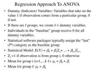
Regression-based Approach for Calculating CBL. Dr. Sunil Maheshwari Dominion Virginia Power. Benefits of Regression Approach. This approach can be used to calculate CBL for both weather-sensitive and non-weather-sensitive loads. The science of regression theory is well developed.

E N D
Regression-based Approachfor Calculating CBL Dr. Sunil Maheshwari Dominion Virginia Power
Benefits of Regression Approach • This approach can be used to calculate CBL for both weather-sensitive and non-weather-sensitive loads. • The science of regression theory is well developed. • Most statistical packages such as SAS, STATA, SPSS, etc. can perform regression analysis. • Regression equations can be easily updated on a periodic basis (perhaps annually).
Description of Regression Approach • The idea is to treat load as a function of explanatory factors such as weather, time of day, day of the week, etc. • Estimate the relationship between load and explanatory variables using a variety of functional forms. • Pick the functional form that gives the highest R-sq adjusted or the lowest Root Mean Squared Error (RMSE)
Functional Forms for Weather-Sensitive Loads Form 1: Load = a + b*CDD + c*HDD Form 2: Load = a+ Σ (bi * CDDi) + Σ (cj * HDDj); Temperature breakpoints to be established based on Regression Analysis Form 3: Load = a+ Σ (bi * CDDi) + Σ (cj * HDDj) + Σ (dk * hourk); In addition to weather, each hour impacts the load as well.
Functional Forms for Non-Weather Sensitive Loads • The following forms may do a good job of estimating CBL for Industrial loads: Form 4: Load = a + Σ (bk * hourk) + Σ (cj * monthj); Form 5: Load = a + b * TimeTrend + Σ (ck * hourk) + Σ (dj * monthj);
Applying Theory into Practice… • For one of our DSR participants (a Building Complex), we estimated the relationship between 2006 hourly Load and Weather using Functional Form 3: Load = a+ Σ (bi * CDDi) + Σ (cj * HDDj) + Σ (dk * hourk); • Following temperature breakpoints were used: • For Heating Degree Days (HDD) – 65, 55, 40, 25 • For Cooling Degree Days (CDD) – 65, 80, 90, 100
Applying Theory into Practice… • We further sliced the data by: • Day type • Weekdays • Weekends and Holidays • Season • Winter – December - March • Summer – June - September • Shoulder – April, May, October, November
Partial Regression Output (Summer, Weekday) regress load cdd_65to80 cdd_80to90 cdd_90to100 cdd_over100 hdd hddsq hour2-hour24 if year==2006 & weekdayflag==1 & holiday==0 & season=="Summer" Source | SS df MS Number of obs = 2040 -------------+------------------------------ F( 28, 2011) = 518.86 Model | 339127510 28 12111696.8 Prob > F = 0.0000 Residual | 46942715.2 2011 23342.9713 R-squared = 0.8784 -------------+------------------------------ Adj R-squared = 0.8767 Total | 386070225 2039 189342.925 Root MSE = 152.78 ------------------------------------------------------------------------------ load | Coef. Std. Err. t P>|t| [95% Conf. Interval] -------------+---------------------------------------------------------------- cdd_65to80 | 33.08646 .9634143 34.34 0.000 31.19707 34.97586 cdd_80to90 | 31.6024 .5931229 53.28 0.000 30.4392 32.7656 cdd_90to100 | 32.58845 .68489 47.58 0.000 31.24528 33.93162 cdd_over100 | (dropped) hdd | -104.137 6.194134 -16.81 0.000 -116.2846 -91.98941 hddsq | 4.866126 .6342737 7.67 0.000 3.622224 6.110028 hour2 | -33.26744 23.44299 -1.42 0.156 -79.24253 12.70765 hour3 | 19.0973 23.452 0.81 0.416 -26.89547 65.09006 hour4 | 25.50128 23.46632 1.09 0.277 -20.51955 71.52211
Predicted Load (CBL) based on 2006 data applied to 2007 data • Using regression parameters from previous slide, predict the load for 2007. • Compare predicted load (CBL) to actual load. • Absolute average % deviation between Actual and Predicted Load was less than 5%. • Regression Equations will be re-estimated every year
Actual Load vs Predicted (CBL) - Summer, Weekday(Absolute Average % Deviation = 3%)
Actual Load vs Predicted (CBL) - Winter, Weekday(Absolute Average % Deviation = 3.6%)
Actual Load vs Predicted (CBL) - Shoulder, Weekday(Absolute Average % Deviation = 3.7%)
Actual Load vs Predicted (CBL) - Weekend/Holiday(Absolute Average % Deviation = 4.7%)
Conclusions • 4 Equations with single variable hourly temperature • Summer, Weekday • Winter, Weekday • Shoulder, Weekday • Weekends / Holidays • Good fit (R-sq adjusted > 78% in all cases). • Simplified calculations, and the regression equations can be easily updated.