Download
1 / 29
290 likes | 296 Vues
Simultaneous Modeling of Developer Behavior and Land Prices in UrbanSim. Daniel Felsenstein Eyal Ashbel. UrbanSim European Users Group meeting, ETH Zurich, 17-18 th March 2008. The Motivation. In UrbanSim, interdependence between developer behavior and land prices is noted.

E N D
Simultaneous Modeling of Developer Behavior and Land Prices in UrbanSim Daniel Felsenstein Eyal Ashbel UrbanSim European Users Group meeting, ETH Zurich, 17-18th March 2008
The Motivation • In UrbanSim, interdependence between developer behavior and land prices is noted. • Interdependence between dev.behav/land prices and h’hold and job location choice, is also noted. • However, in the model developer behavior and land prices are modeled independently. • In practice, the two occur simultaneously
Motivation cont. • UrbanSim models assumes prices are exogenous to interaction between buyers and sellers (their individual transactions are too small to affect aggregate prices). • But much urban economics points to endogeneity issue: developer behavior depends on land prices and land prices depend on developer behavior • Issue of endogeneity means dealing with: • Correct identification of models (error structures) • Instrumentation • Dynamics
Motivation cont 2. • Dynamics in current land price model: cross-section simulation of end-of-the-year-prices based on updated cell characteristics (from developer model, h’hold and jobs location choices and transport model). • These land prices then influence h’holds, jobs, developer behavior in next year: back-door endogeneity? • Prices also fixed by expectations of price (rational expectations world)
S' (π+1= π) S'' (π+1> π) A B D Theory Relative Price Quantity
(–) (+) Supply Demand Z, X = vectors of variables that cause supply/demand curves to shift general price is sum of parcel prices. Equilibrium
Adding in future expectations (e) Rational Expectations Assumptions: expected price + error term E(vit+1)=0 people do not expect to err. E(vit+1it)=0 = current information factor – instrument for future relative prices.
Adding time factor to future expectations: yt=xt+[yt+1-vt+1]+ut E(vt+1,ut)=0 =xt+yt+1+ut- vt+1 E(yet+1)<0 IV: yt+1 , xt , vt+1
Estimation Strategy Maddala (1983): simultaneous equations Use probit two-stage least squares (P2SLS) CDSIMEQ routine (STATA Journal 2003) Land price model (OLS) Developer model (probit)
Simultaneous equations • y*2 is not observed, rewrite (1) and (2) as • Estimate reduced form • Extract predicted values • Plug-in fitted values and adjust covariance matrix
In our case:y1 observed (continuous)- land prices y2 dichotomous – developer behavior Simultaneous equations:
As is not observed (ie only observed as a dichotomous variable), equations (1) and (2) are re-written: This has implications for standard errors that will need to be corrected later on.
Two-stage Estimation Stage 1: (estimated by OLS and probit): models fitted using all exogenous variables. Predicted values obtained. X= matrix of all exogenous variables Π1’Π2,= vectors of parameters to be estimated From these reduced-form estimates, predicted values from each model are obtained for use in Stage 2.
Two-stage Estimation cont. Stage 2: (estimated by OLS and probit): original endogenous variables in (3) and (4) are replaced by their fitted values from (7) and (8). Finally, need correction for standard errors (adjustment of the variance- covariance matrix) as models based on and not on the appropriate
Tel Aviv Metropolitan Area • 1,683 sq km. • Three million inhabitants. • One million employees • 49 % National GNP. • 60 local authorities (city governments)
Non-residential • Non-resid sq m: development starts later but reaches more extreme values • Similar trends to individual model estimation. Accentuated suburban non-residential development • Simultaneous estimation makes for more extreme values in non- resid land prices. Less smooth price gradient
Residential • Simultaneous estimation predicts more population deconcentration. • Residential land values are estimated to be higher in suburban locations than in CBD (using simultaneous estimation) • Individual estimation gives opposite picture: higher residential prices closer to CBD
Results for Individual Local Authorities • Results tend to stabilize over the longer term (2020) • Households data: simultaneous estimation generally yields higher outcomes (positive deltas) than individual estimation. • Changes in attributes of cells: estimates of changes in non-residential cells (units, area) much more volatile than for residential cells. Confirms results relating to land values. • Southern local authorities estimated gains much more in non-residential units than in residential (implications for fiscal independence).
Conclusions • Avoiding endogeneity in price fixing= the easy way out? • Explicit treatment of prices in UrbanSim- can this be improved? (Prices respond at the end of the year to grid cell characteristics of location, balance of supply an demand at each location) • Price expectations need to be included (need credible instrument) • Is this more suited to UrbanSim4?