Download
1 / 20
200 likes | 204 Vues
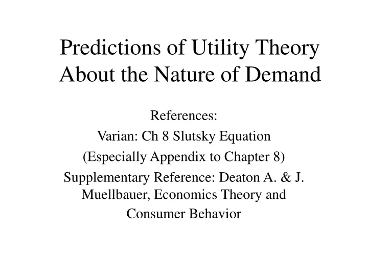
Predictions of Utility Theory About the Nature of Demand. References: Varian: Ch 8 Slutsky Equation (Especially Appendix to Chapter 8) Supplementary Reference: Deaton A. & J. Muellbauer, Economics Theory and Consumer Behavior. Predictions of Utility Theory About the Nature of Demand.

E N D
Predictions of Utility Theory About the Nature of Demand References: Varian: Ch 8 Slutsky Equation (Especially Appendix to Chapter 8) Supplementary Reference: Deaton A. & J. Muellbauer, Economics Theory and Consumer Behavior
Predictions of Utility Theory About the Nature of Demand • Have already determined 2 properties of demand function which follow from the axioms (or properties) 1-7 we have assumed about the utility function. • We have also seen how the effect of a price change can be separated into either Hicksian or Slutsky Income & Substitution effects.
Testable Predictions and the Theory • The two properties already identified, the Adding-up and Cournot conditions gave us firm measures which we could use to test consumer theory. • The next piece of theory we developed suggested that both the Hicksian and Slutsky Pure substitution effects are always negative. This is a prediction of our theory. • Is the negativity of the pure substitution effect similarly testable given that it is not directly observable.
Properties of Demand Function: No. 3 The Pure Substitution effect isNegative (Strictly it is Never Positive)
The SLUTSKY EQUATION xD = x (Px, Py, M) First, although this is known as the Slutsky equation, we will look at the Hicksian case where we compensate the consumer for the change in prices by placing her back on her original indifference curve.
Income and substitution effects: normal good g h Units of good Y f I1 I2 I3 I4 I5 B2 B2a B1 I6 QX3 QX1 QX2 Substitution effect Income effect Units of Good X Units of Good X
The SLUTSKY EQUATION xD = x (Px, Py, m) We know that for a change in the price of x, Overall effect = Substitution effect (U held constant) + income effect Thus: But M= Pxx, + Py,y So, xD= x (Px, Py, Pxx + Pyy)
So, Called the Hicks - Slutsky Decomposition
The Slutsky Equation or The Hicks - Slutsky Decomposition This says that the pure substitution effect is a combination of the price effect and the income effect. While we cannot observe the variable on the LHS, we can observe everything on the RHS. So we can test the prediction that the pure substitution effect is negative by measuring
Third Testable Prediction: • The Pure Substitution Effect is Non-Positive
The Slutsky Equation or The Hicks - Slutsky Decomposition If it is true that the pure substitution effect is always negative, then we know from the expression above that as long as the good is normal (that is, mi implies x i) Then the demand curve slopes down.
The SLUTSKY EQUATION xD = x (Px, Py, M) Technically, as we have already said, this measures the Hicksian effect rather than the Slutsky effect, but we can write a similar expression for Slutsky. Recall, with Slutsky we compensate the consumer for the change in prices by allowing him to purchase the original bundle.
Income and substitution effects: Slutsky (Solid line) g’ h Units of good Y f I1 I2 I3 I4 I5 B2 B1 I6 B2a QX2 QX3 QX1 Substitution effect Income effect Units of Good X Units of Good X
To represent this we only have to make a minor qualification to the equation: Hence called the Hicks - Slutsky Decomposition
Hicks - Slutsky Decomposition • In practice for very small changes in prices the Hicksian and Slutsky effects are essentially the same. • For the most part, the terms we use to test the theory are derivatives of an estimated function and the Slutsky and Hicksian effects are synonymous • However, if we are looking at compensating government tax changes for example then the difference is important.
Note: Main text in Varian uses the terminology, xs , and discusses the concept in terms of changes. You can use this if you want, but prefer to use the derivative terms as in the appendix to the chapter. The Varian (appendix) expression is (The two goods are x1 and x2) :
Finally, we can write The Hicks - Slutsky Decomposition in Elasticity Form
Slutsky Summary: • Although the Pure Substitution is unobservable the Slutsky Equation tell us that we can test whether it is negative (not positive) by checking the magnitude of three observable phenomenon: • the elasticity of demand for x, • the share of x in expenditurte • and the income elasticity of demand for x.
Summaryof Properties • This section has identified three properties of demand functions (there are others): 1. The Adding-Up Condition 2. The Cournot Condition 3. The Non-Positive Pure Substitution Effect
Summary of Course So far: • So after a lot of hard work we have identified 7 axioms we would like to assume preferences follow to generate well behaved demand functions. • As a consequence we have identified three properties we would like these demand curves to obey • If demand functions fit these properties are assumptions about preferences are reasonable. • Do They? Well….., yes and no