Download
1 / 48
480 likes | 486 Vues
Visual Object Recognition. Bastian Leibe & Computer Vision Laboratory ETH Zurich Chicago, 14.07.2008. Kristen Grauman Department of Computer Sciences University of Texas in Austin. Outline. Detection with Global Appearance & Sliding Windows

E N D
Visual Object Recognition Bastian Leibe & Computer Vision Laboratory ETH Zurich Chicago, 14.07.2008 Kristen Grauman Department of Computer Sciences University of Texas in Austin
Outline Detection with Global Appearance & Sliding Windows Local Invariant Features: Detection & Description Specific Object Recognition with Local Features ― Coffee Break ― Visual Words: Indexing, Bags of Words Categorization Matching Local Features Part-Based Models for Categorization Current Challenges and Research Directions 2 K. Grauman, B. Leibe
Detection via classification: Main idea Basic component: a binary classifier Car/non-car Classifier Yes, car. No, not a car. K. Grauman, B. Leibe
Detection via classification: Main idea If object may be in a cluttered scene, slide a window around looking for it. Car/non-car Classifier K. Grauman, B. Leibe
Car/non-car Classifier Detection via classification: Main idea Fleshing out this pipeline a bit more, we need to: • Obtain training data • Define features • Define classifier Training examples Feature extraction K. Grauman, B. Leibe
Detection via classification: Main idea • Consider all subwindows in an image • Sample at multiple scales and positions • Make a decision per window: • “Does this contain object category X or not?” • In this section, we’ll focus specifically on methods using a global representation (i.e., not part-based, not local features). 6 K. Grauman, B. Leibe
Feature extraction Feature extraction: global appearance • Simple holistic descriptions of image content • grayscale / color histogram • vector of pixel intensities K. Grauman, B. Leibe
Eigenfaces: global appearance description An early appearance-based approach to face recognition Generate low-dimensional representation of appearance with a linear subspace. Mean Eigenvectors computed from covariance matrix Training images Project new images to “face space”. Recognition via nearest neighbors in face space ... + + + + Mean Turk & Pentland, 1991 K. Grauman, B. Leibe
Feature extraction: global appearance • Pixel-based representations sensitive to small shifts • Color or grayscale-based appearance description can be sensitive to illumination and intra-class appearance variation Cartoon example: an albino koala K. Grauman, B. Leibe
Gradient-based representations • Consider edges, contours, and (oriented) intensity gradients K. Grauman, B. Leibe
Gradient-based representations: Matching edge templates • Example: Chamfer matching Distance transform Input image Edges detected Template shape Best match At each window position, compute average min distance between points on template (T) and input (I). Gavrila & Philomin ICCV 1999 K. Grauman, B. Leibe
Gradient-based representations: Matching edge templates • Chamfer matching Hierarchy of templates Gavrila & Philomin ICCV 1999 K. Grauman, B. Leibe
Gradient-based representations • Consider edges, contours, and (oriented) intensity gradients • Summarize local distribution of gradients with histogram • Locally orderless: offers invariance to small shifts and rotations • Contrast-normalization: try to correct for variable illumination K. Grauman, B. Leibe
Gradient-based representations:Histograms of oriented gradients (HoG) Map each grid cell in the input window to a histogram counting the gradients per orientation. Code available: http://pascal.inrialpes.fr/soft/olt/ Dalal & Triggs, CVPR 2005 K. Grauman, B. Leibe
Gradient-based representations:SIFT descriptor Local patch descriptor (more on this later) Code: http://vision.ucla.edu/~vedaldi/code/sift/sift.html Binary: http://www.cs.ubc.ca/~lowe/keypoints/ Lowe, ICCV 1999 K. Grauman, B. Leibe
Gradient-based representations:Biologically inspired features Convolve with Gabor filters at multiple orientations Pool nearby units (max) Intermediate layers compare input to prototype patches Serre, Wolf, Poggio, CVPR 2005 Mutch & Lowe, CVPR 2006 K. Grauman, B. Leibe
Gradient-based representations:Rectangular features Compute differences between sums of pixels in rectangles Captures contrast in adjacent spatial regions Similar to Haar wavelets, efficient to compute Viola & Jones, CVPR 2001 K. Grauman, B. Leibe
Gradient-based representations:Shape context descriptor Count the number of points inside each bin, e.g.: Count = 4 ... Count = 10 Log-polar binning: more precision for nearby points, more flexibility for farther points. Local descriptor (more on this later) Belongie, Malik & Puzicha, ICCV 2001 K. Grauman, B. Leibe
Classifier construction Image feature How to compute a decision for each subwindow? K. Grauman, B. Leibe
0.1 0.05 0 0 10 20 30 40 50 60 70 1 0.5 0 0 10 20 30 40 50 60 70 Discriminative vs. generative models Generative: separately model class-conditional and prior densities image feature Discriminative: directly model posterior x = data image feature Plots from Antonio Torralba 2007 K. Grauman, B. Leibe
Discriminative vs. generative models • Generative: • + possibly interpretable • + can draw samples • - models variability unimportant to classification task • - often hard to build good model with few parameters • Discriminative: • + appealing when infeasible to model data itself • + excel in practice • - often can’t provide uncertainty in predictions • - non-interpretable K. Grauman, B. Leibe
Discriminative methods Neural networks Nearest neighbor 106 examples LeCun, Bottou, Bengio, Haffner 1998 Rowley, Baluja, Kanade 1998 … Shakhnarovich, Viola, Darrell 2003 Berg, Berg, Malik 2005... Conditional Random Fields Support Vector Machines Boosting Guyon, Vapnik Heisele, Serre, Poggio, 2001,… Viola, Jones 2001, Torralba et al. 2004, Opelt et al. 2006,… McCallum, Freitag, Pereira 2000; Kumar, Hebert 2003 … K. Grauman, B. Leibe Slide adapted from Antonio Torralba
Boosting • Build a strong classifier by combining number of “weak classifiers”, which need only be better than chance • Sequential learning process: at each iteration, add a weak classifier • Flexible to choice of weak learner • including fast simple classifiers that alone may be inaccurate • We’ll look at Freund & Schapire’s AdaBoost algorithm • Easy to implement • Base learning algorithm for Viola-Jones face detector K. Grauman, B. Leibe
AdaBoost: Intuition Consider a 2-d feature space with positive and negative examples. Each weak classifier splits the training examples with at least 50% accuracy. Examples misclassified by a previous weak learner are given more emphasis at future rounds. Figure adapted from Freund and Schapire K. Grauman, B. Leibe
AdaBoost: Intuition K. Grauman, B. Leibe
AdaBoost: Intuition Final classifier is combination of the weak classifiers K. Grauman, B. Leibe
AdaBoost Algorithm Start with uniform weights on training examples {x1,…xn} Evaluate weighted error for each feature, pick best. Incorrectly classified -> more weight Correctly classified -> less weight Final classifier is combination of the weak ones, weighted according to error they had. Freund & Schapire 1995
Cascading classifiers for detection For efficiency, apply less accurate but faster classifiers first to immediately discard windows that clearly appear to be negative; e.g., • Filter for promising regions with an initial inexpensive classifier • Build a chain of classifiers, choosing cheap ones with low false negative rates early in the chain Fleuret & Geman, IJCV 2001 Rowley et al., PAMI 1998 Viola & Jones, CVPR 2001 Figure from Viola & Jones CVPR 2001 K. Grauman, B. Leibe
Example: Face detection • Frontal faces are a good example of a class where global appearance models + a sliding window detection approach fit well: • Regular 2D structure • Center of face almost shaped like a “patch”/window • Now we’ll take AdaBoost and see how the Viola-Jones face detector works K. Grauman, B. Leibe
Feature extraction “Rectangular” filters • Feature output is difference between adjacent regions Value at (x,y) is sum of pixels above and to the left of (x,y) • Efficiently computable with integral image: any sum can be computed in constant time • Avoid scaling images scale features directly for same cost Integral image Viola & Jones, CVPR 2001 K. Grauman, B. Leibe
Large library of filters • Considering all possible filter parameters: position, scale, and type: • 180,000+ possible features associated with each 24 x 24 window Use AdaBoost both to select the informative features and to form the classifier Viola & Jones, CVPR 2001
Want to select the single rectangle feature and threshold that best separates positive (faces) and negative (non-faces) training examples, in terms of weighted error. AdaBoost for feature+classifier selection Resulting weak classifier: For next round, reweight the examples according to errors, choose another filter/threshold combo. … Outputs of a possible rectangle feature on faces and non-faces. Viola & Jones, CVPR 2001
Viola-Jones Face Detector: Summary • Train with 5K positives, 350M negatives • Real-time detector using 38 layer cascade • 6061 features in final layer • [Implementation available in OpenCV: http://www.intel.com/technology/computing/opencv/] Train cascade of classifiers with AdaBoost Apply to each subwindow Faces New image Selected features, thresholds, and weights Non-faces K. Grauman, B. Leibe
Viola-Jones Face Detector: Results First two features selected K. Grauman, B. Leibe
Profile Features Detecting profile faces requires training separate detector with profile examples.
Viola-Jones Face Detector: Results Paul Viola, ICCV tutorial
Example application Frontal faces detected and then tracked, character names inferred with alignment of script and subtitles. Everingham, M., Sivic, J. and Zisserman, A."Hello! My name is... Buffy" - Automatic naming of characters in TV video,BMVC 2006. http://www.robots.ox.ac.uk/~vgg/research/nface/index.html 40 K. Grauman, B. Leibe
Pedestrian detection • Detecting upright, walking humans also possible using sliding window’s appearance/texture; e.g., SVM with Haar wavelets [Papageorgiou & Poggio, IJCV 2000] Space-time rectangle features [Viola, Jones & Snow, ICCV 2003] SVM with HoGs [Dalal & Triggs, CVPR 2005] K. Grauman, B. Leibe
Highlights • Sliding window detection and global appearance descriptors: • Simple detection protocol to implement • Good feature choices critical • Past successes for certain classes K. Grauman, B. Leibe
Limitations • High computational complexity • For example: 250,000 locations x 30 orientations x 4 scales = 30,000,000 evaluations! • If training binary detectors independently, means cost increases linearly with number of classes • With so many windows, false positive rate better be low K. Grauman, B. Leibe
Limitations (continued) • Not all objects are “box” shaped K. Grauman, B. Leibe
Limitations (continued) • Non-rigid, deformable objects not captured well with representations assuming a fixed 2d structure; or must assume fixed viewpoint • Objects with less-regular textures not captured well with holistic appearance-based descriptions K. Grauman, B. Leibe
Limitations (continued) • If considering windows in isolation, context is lost Sliding window Detector’s view Figure credit: Derek Hoiem K. Grauman, B. Leibe
Limitations (continued) • In practice, often entails large, cropped training set (expensive) • Requiring good match to a global appearance description can lead to sensitivity to partial occlusions K. Grauman, B. Leibe Image credit: Adam, Rivlin, & Shimshoni
Outline Detection with Global Appearance & Sliding Windows Local Invariant Features: Detection & Description Specific Object Recognition with Local Features ― Coffee Break ― Visual Words: Indexing, Bags of Words Categorization Matching Local Features Part-Based Models for Categorization Current Challenges and Research Directions 48 K. Grauman, B. Leibe