Download
1 / 58
580 likes | 584 Vues
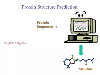
This chapter explores the prediction of protein and RNA structures using computational methods such as neural networks, hidden Markov models, and evolutionary computation. It covers topics like amino acids, secondary structure prediction, tertiary and quaternary structure, and algorithms for protein folding.

E N D
Chapter 7Protein and RNA Structure Prediction 暨南大學資訊工程學系 黃光璿 2004/05/24
Proteins • Built from a repertoire of 20 amino acids
胺基酸 • 中心碳 • 胺基(NH2) • COOH • 氫(H) • 側鏈(side chain, R)
pH, pKa, and pI • pH • -log [H+] • pKa • = pH ~ half of the amino acid residues will dissociate (釋放出H+). • pI • = pH, isoelectric point for protein
Ramachandran Plot N:藍 C:黑 O:紅 H:白
二級結構(Secondary Structure) • Alpha helix
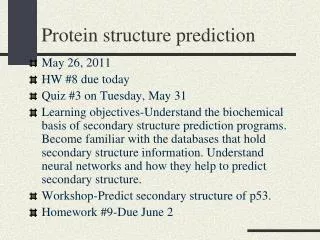
7.3.2 Accuracy of Prediction • Computational methods • neural network • discrete-state models • hidden Markov models • nearest neighbor classification • evolutionary computation
PHD, Predator • structure prediction algorithms • accuracies in the range 70% ~ 75%
Identifying Alpha Helices • Find all regions where four out of six have P(a)>100. • Extend the regions until four with P(a) < 100 in both directions. • If ΣP(a) > ΣP(b) and the stretch >5, then it is identified as a helix.
Identifying Beta Sheets • Find all regions where four out of six have P(b)>100. • Extend the regions until four with P(b) < 100 in both directions. • If ΣP(b) > ΣP(a) and the average value of P(b) over the stretch >100, then it is identified as a helix.
Resolving Overlapping Regions • Identified as helix if ΣP(a) > ΣP(b), as sheet if ΣP(b) > ΣP(a) over the overlapping regions.
Identifying Turns • Let P(t) = f(i)xf(i+1)xf(i+2)xf(i+3) for each position i. • Identify as a turn if • P(t) > 0.000075; • The average of P(turn) over the four residues > 100; • ΣP(a) < ΣP(turn) > ΣP(b) over the four residues.
7.3.4 GOR Method • on a window of 17 residues
折疊成立體的形狀 三級結構(Tertiary Structure)
四級結構(Quaternary Structure) • 數個三級結構結合成具有功能的大分子 人類的血球蛋白
Driving Forces for Folding • electrostatic forces • hydrogen bonds • van der Waals forces • disulfide bonds • solvent interactions
7.4.1 Hydrophobicity (疏水性) • hydrophobic collapse • Tend to keep polar, charged residues on the surface. • The class of membrane-integral proteins is an exception.
sickle-cell anemia (鐮狀細胞性貧血) • human hemoglobin: 2 alpha & 2 beta globins • charged glutamic acid residue hydrophobic valine residues
7.4.3 Active Structures vs Most Stable Structures • Natural selection favors proteins that are both active and robust.
Levinthal Paradox • in 1968 • 100 residues, each assume 3 different conformations • 3100 ~ 5x1047 possibilities • Suppose it takes 10-13 s for one trial. • Proteins fold by progressive stabilization of intermediates rather than by random search.
7.5 Algorithms for Modeling Protein Folding • Lattice Models • Off-Lattice Models
7.5.1 Lattice Models • Reduce the search space and make computing tractable. Minimize free energy conformation
HP-model • hydrophobic-polar model • Scoring is based on hydrophobic contacts. • Maximize the H-to-H contacts. • Fig. 7.8
7.5.2 Off-Lattice Models • Use RMSD (root mean square deviation) to measure the accuracy. • Determine Φ and Ψin the allowable region of the Ramachandran plot.
7.5.3 Energy Functions and Optimization • Problems • The exact forces that drive the folding process are not well understood. • It is too computationally expensive.
Summary • model • representation • scoring function • search (optimization) • Folding@Home (V. Pande, Stanford)