Download

1 / 50
671 likes | 1.73k Vues
Canonical correlation. Return to MR. Previously, we’ve dealt with multiple regression, a case where we used multiple independent variables to predict a single dependent variable

E N D
Return to MR • Previously, we’ve dealt with multiple regression, a case where we used multiple independent variables to predict a single dependent variable • We came up with a linear combination of the predictors that would result in the most variance accounted for in the dependent variable (maximize R2) • We have also introduced PC regression, in which linear combinations of the predictors which account for all the variance in the predictors can be used in lieu of the original variables • Reason? • Dimension reduction: select only the best components • Independence of predictors: solves collinearity issue
More DVs • The problem posed now is what to do if we had multiple dependent variables • How could we come up with a way to understand the relationship between a set of predictors and DVs? • Canonical Correlation measures the relationship between two sets of variables • Example: looking to see if different personality traits correlate with performance scores for a variety of tasks
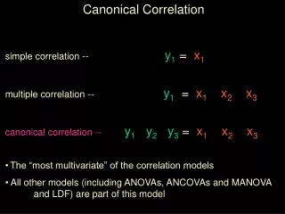
What is Canonical Correlation? • CC extends bivariate correlation, allowing 2+ continuous IVs (on left) with 2+ continuous DVs (variables on right). • Focus is on correlations & weights • Main question: How are the best linear combinations of predictors related to the best linear combinations of the DVs?
Analysis • In CC, there are several layers of analysis: • Correlation between pairs of canonical variates • Loadings between IVs & their canonical variates (on left) • Loadings between DVs & their canonical variates (on right) • Adequacy • Communalities • Other • Redundancy between IVs & can. variates on other (right) side • Redundancy between DVs & can. variates on other (left) side • As we will discuss later, these are problematic
When to use? • As exploratory tool to see if two sets of continuous variables are related • If significant overall shared variance (i.e., by 1- 2 and F-test), several layers of analysis can explore variables & variates involved • In a modeling type approach where you have a theoretical reason for considering the variables as sets, and that one predicts another • See if one set of 2+ variables relates longitudinally across two time points • Variables at t1 are predictors; same variables at t2 are DVs • See layers of analysis for tentative causal evidence
Compare to MR • With canonical correlation we will again (like in MR) be creating linear combinations for our sets of variables • In MR, the multiple correlation coefficient was between the predicted values created by the linear combination of predictors (i.e. the composite) and the dependent variable • R2 = square of multiple correlation
Canonical Correlation • Creating linear composites of our respective variable sets (X,Y): • Creating some single variable that represents the Xs and another single variable that represents the Ys. • Given a linear combination of X variables: F = f1X1 + f2X2 + ... + fpXp and a linear combination of Y variables: G = g1Y1 + g2Y2 + ... + gqYq The first canonical correlation is: The maximum correlation coefficient between F and G, for all F and G • The correlation we are interested in here will be between the linear combinations (variates) created for both sets of variables • However now there will be the possibility for several ways in which to combine the variables that provide a useful interpretation of the relationship
Canonical Correlation: Layers Micro Step 2: Macro: Correlate Canonical Variates (Vs & Ws) R2c1 R E D U N D A N C Y W1 X1 V1 Y1 R2c2 X2 W2 V2 Y2 R2c3 X3 V3 W3 Y3 X4 Micro Step 1: Loadings
Some initial terms • Variables • Those measurements recorded in the dataset • Canonical Variates • The linear combination of the sets of variables (predictor and DV) • One variate for each set of variables • Canonical correlation • The correlation between variates • Pairs of Canonical Variates • As mentioned, we may have more than one pair of linear combinations that provide an interesting measure of the relationship
Background • Canonical Correlation is one of the most general multivariate forms – multiple regression, discriminate function analysis and MANOVA are all special cases of it • As the basic output of regression and ANOVA are equivalent, so too is the case here between canonical correlation and regression • Example: CanCorr squared between predictor set and a lone DV = R2 from multiple regression • Only one solution • The number of canonical variate pairs you can have is equal to the number of variables in the smaller set • When you have many variables on both sides of the equation you end up with many canonical correlations. • Arranged in descending order, in most cases the first one or two will be the ones of interest.
Things to think about • Number of canonical variate pairs • How many prove to be statistically/practically significant? • Interpreting the canonical variates • Where is the meaning in the combinations of variables created? • Importance of canonical variates • How strong is the correlation between the canonical variates? • What is the nature of the variate’s relation to the individual variables in its own set? The other set? • Canonical variate scores • If one did directly measure the variate, what would the subjects’ scores be?
Limitations • The procedure maximizes the correlation between the linear combination of variables, however the combination may not make much sense theoretically • Nonlinearity poses the same problem as it does in simple correlation i.e. if there is a nonlinear relationship between the sets of variables the technique is not designed to pick up on that • Cancorr is very sensitive to data involved i.e. influential cases and which variables are chosen or left out of analysis can have dramatic effects on the results just like they do elsewhere • Correlation, as we know, does not automatically imply causality • It is a necessary but not sufficient condition for causality • Being a simple correlation in the end, cancorr is often thought of as a descriptive procedure
Practical concerns • Sample size • Number of cases required ≈ 10-20 per variable in the social sciences where typical reliability is .80 • More if they are less reliable, or more than one canonical function is interpreted. • Normality • Normality is not specifically required if purely used descriptively • But using continuous, normally distributed data will make for a better analysis • If used inferentially, significance tests are based on multivariate normality assumption • All variables and all linear combinations of variables are normally distributed
Practical concerns • Linearity • Linear relationship assumed for all variables in each set and also between sets • Homoscedasticity • Variance for one variable is similar for all levels of another variable • Can be checked for all pairs of variables within and between sets. • One may assess these assumptions at the variate level after a preliminary CC has been run, much like we do with MR
Practical concerns • Multicollinearity/Singularity • Having variables that are too highly correlated or that are essentially a linear combination of other variables can cause problems in computation • Check Set 1 and Set 2 separately • Run correlations and use the collinearity diagnostics function in regular multiple regression • Outliers • Check for both univariate and multivariate outliers on both set 1 and set 2 separately
So how does it work? • Canonical Correlation uses the correlations from the raw data and uses this as input data • You can actually put in the correlations reported in a study and perform your own canonical correlation (e.g. to check someone else’s results) • Or any other analysis for that matter
Data • The input correlation setup is • The canonical correlation matrix is the product of four correlation matrices, between DVs (inverse of Ryy,), IVs (inverse of Rxx), and between DVs and IVs • It also can be thought of as a product of regression coefficients for predicting Xs from Ys, and Ys from Xs
What does it mean? • In this context the eigenvalues of that R matrix represent the percentage of overlapping variance between the canonical variate pairs • To get the canonical correlations, you get the eigenvalues of R and take the square root • The eigenvector corresponding to each eigenvalue is transformed into the coefficients that specify the linear combination that will make up a canonical variate
Canonical Coefficients • Two sets of canonical coefficients (weights) are required • One set to combine the Xs • One to combine the Ys • Same interpretation as regression coefficients
Is it statictically significant? • Testing Canonical Correlations • There will be as many canonical correlations as there are variables in the smaller set • Not all will be statistically significant • Bartlett’s Chi Square test (Wilk’s on printouts) • Tests whether an eigenvalue and the ones that follow are significantly different than zero • It is possible this test would be significant even though a test for the correlation itself would not be
Is it really significant? • So again, one may ask whether ‘significantly different from zero’ is an interesting question • As it is simply a correlation coefficient, one should be more interested in the size of the effect, more than whether it is different from zero (it always is)
Variate Scores • Canonical Variate Scores • Like factor scores (we’ll get there later) • What a subject would score if you could measure them directly on the canonical variate • The values on a canonical variable for a given case, based on the canonical coefficients for that variable. • Canonical coefficients are multiplied by the standardized scores of the cases and summed to yield the canonical scores for each case in the analysis
Loadings rX1 \rX2 X1 ry1 ry2 W1 Y1 V1 X2 rX3 rX4 ry3 Y2 X3 Y3 X4 Loadings (structure coefficients) • Loadings or structure coefficients • Key question: how well do the variate(s) on either side relate to their own set of measured variables? • Bivariate correlation between a variable and its respective variate • Would equal the canonical coefficients if all variables were uncorrelated with one another • Its square is the proportion of variance linearly shared by a variable with the variable’s canonical composite • Found by multiplying the matrix of correlations between variables in a set by the matrix of canonical coefficients
Loadings vs. canonical (function) coefficients • Which for interpretation? • Recall that coming up with the best correlation may result in variates which are not exactly interpretable • One might think of the canonical coefficients as regarding the computation of the variates, while loadings refer to the relationship of the variables to the construct created • Use both for a full understanding of what’s going on
Canonical communality coefficient Sum of the squared structure coefficients (loadings) across all variates for a given variable. Measures how much of a given original variable's variance is reproducible from the canonical variates. If looking at all variates it will equal one, however typically we are often dealing with only those retained for interpretation, and so it may be given for those that are interpreted Canonical variate adequacy coefficient Average of all the squared structure coefficients (loadings) for one set of variables with respect to their canonical variate. A measure of how well a given canonical variable represents the variance in that set of original variables. X1 V1 V2 V3 X1 V1 X2 X3 X4 More coefficients
Redundancy • Redundancy • Key question: how strongly do the individual measured variables on one side of the model relate to the variate on the other side? • Product of the mean squared structure coefficient (i.e. the adequacy coefficient) for a given canonical variate times the squared canonical correlation coefficient. • Measures how much of the average proportion of variance of the original variables of one set may be ‘predicted’ from the variables in the other set • High redundancy suggests, perhaps, high ability to predict X1 Y1 V1 W1 X2 Y2 X3 Y3 X4
Redundancy • Canonical correlation reflects the percent of variance in the dependent canonical variate explained by the predictor canonical variate • Used when exploring relationships between the independent and the dependent set of variables. • Redundancy has to do with assessing the effectiveness of the canonical analysis in capturing the variance of the original variables. • One may think of redundancy analysis as a check on the meaning of the canonical correlation. • Redundancy analysis (from SPSS) gives a total of four measures • The percent of variance in the set of original individual dependent variables explained by the independent canonical variate (adequacy coefficient for the independent variable set) • A measure of how well the independent canonical variate predicts the values of the original dependent variables • A measure of how well the dependent canonical variate predicts the values of the original dependent variables (adequacy coefficient for the dependent variable set) • A measure of whether the dependent canonical variate predicts the values of the original independent variables
CCA: the mommy of statistical analysis • Just as a t-test is a special case of Anova, and Anova and Ancova are special cases of regression, regression analysis is a special case of CCA • If one were to conduct an MR and CCA on the same data R2 = R2c1 • Canonical coefficients = Beta weights/Multiple R • Almost all of the classical methods you have learned thus far are canonical correlations in this sense • And you thought stats was hard!
Why not more CCA? • From Thompson (1980): • “One reason why the technique is [somewhat] rarely used involves the difficulties which can be encountered in trying to interpret canonical results… The neophyte student of CCA may be overwhelmed by the myriad coefficients which the procedure produces… [But] CCA produces results which can be theoretically rich, and if properly implemented, the procedure can adequately capture some of the complex dynamics involved in reality.” • Thompson (1991): • “CCA is only as complex as reality itself”
Guidelines for interpretation • Use the R2c and significance tests to determine the canonical functions to interpret • More so the former • Furthermore, the significance tests are not tests of the single Rc but of that one and the rest that follow • Use both the canonical and structure coefficients to help determine variable contribution • Note that such redundancy coefficients are not truly part of the multivariate nature of the analysis and so not optimized1
Guidelines for interpretation • Use the communality coefficients to determine which variables are not contributing to the CCA solution • Note that measurement error attenuates Rc and this is not accounted for by this analysis (compare Factor analysis) • Validate and or Replicate • Use large samples for validation • Can apply Wherry’s correction and get Adusted Rc
Example in SPSS • Software: SPSS • Dataset: GSS_Subset • Burning research question: Does family income, education level, and ‘science background’ predict musical preference? • SPSS does not provide a means for conducting canonical correlation through the menu system • SPSS does however provide a macro to pull it off • “Canonical correlation.sps” in the SPSS folder on your computer
Syntax • The syntax • Set1 IVs, Set2 DVs • Not much to it, and most programs are similar in this regard
Output • Unfortunately the output isn’t too pretty and some of it will not be visible at first • Might be easiest to double click the object, highlight all the output and put into word for screen viewing
Variable correlations • The initial output involves correlations among the variables for each set, then among all six variables • Note that musical preference is scored so that lower scores indicate ‘me likey’ (1- like, 4 dislike) • Scitest4 is “Humans Evolved From Animals” (1- Definitely true, 4- Definitely not • Not too much relationship between those in Set2 • Negative relationship between classical and educ indicates more education associated with more preference for classical music Correlations for Set-1 educ income91 scitest4 educ 1.0000 .4036 -.2438 income91 .4036 1.0000 -.0819 scitest4 -.2438 -.0819 1.0000 Correlations for Set-2 country classicl rap country 1.0000 -.1133 -.0570 classicl -.1133 1.0000 .0222 rap -.0570 .0222 1.0000 Correlations Between Set-1 and Set-2 country classicl rap educ .2249 -.3387 -.0221 income91 .0961 -.1676 .0754 scitest4 -.1312 .0755 .0872
Canonical correlations • Next we have the canonical correlations among the three pairs of canonical variates created • The first is always of most interest, and here probably the only one Canonical Correlations 1 .390 2 .137 3 .042
Significance tests • Note again what the significance tests are actually testing • So are first says that there is some difference from zero in there somewhere • The second suggests there is some difference from zero among the last two canonical correlations • Only the last is testing the statistical significance of one correlation Test that remaining correlations are zero: Wilk's Chi-SQ DF Sig. 1 .831 206.694 9.000 .000 2 .980 22.956 4.000 .000 3 .998 1.926 1.000 .165
Canonical coefficients • Next we have the raw and standardized coefficients used to create the canonical variates • Again, these have the same interpretation as regression coefficients, and are provided for each pair of variates created, regardless of the correlation’s size or statistical significance Standardized Canonical Coefficients for Set-1 1 2 3 educ -.937 .073 -.616 income91 -.084 -.699 .836 scitest4 .092 -.780 -.668 Raw Canonical Coefficients for Set-1 1 2 3 educ -.310 .024 -.204 income91 -.016 -.131 .156 scitest4 .082 -.690 -.591 Standardized Canonical Coefficients for Set-2 1 2 3 country -.500 .362 .797 classicl .811 .306 .512 rap .011 -.881 .477 Raw Canonical Coefficients for Set-2 1 2 3 country -.463 .336 .739 classicl .662 .250 .418 rap .010 -.803 .435
Canonical loadings • Now we get to the particularly interesting part, the structure coefficients • We get correlations between the variables and their own variate as well as with the other variate • Mostly interested in the loading on their own • Most of these are not too different from the canonical coefficients, however they increasingly vary with increased intercorrelations among the variables in the set • Only if they are completely uncorrelated will the canonical coefficients = canonical loadings • Recall how there wasn’t much correlation among our music scores, and compare the loadings to the canonical coefficients Canonical Loadings for Set-1 1 2 3 educ -.993 -.019 -.115 income91 -.470 -.606 .642 scitest4 .328 -.741 -.586 Cross Loadings for Set-1 1 2 3 educ -.387 -.003 -.005 income91 -.183 -.083 .027 scitest4 .128 -.101 -.024 Canonical Loadings for Set-2 1 2 3 country -.592 .378 .712 classicl .868 .245 .432 rap .057 -.895 .443 Cross Loadings for Set-2 1 2 3 country -.231 .052 .030 classicl .338 .033 .018 rap .022 -.122 .018
Canonical loadings • For our predictor variables, education and income load most strongly, but belief in evolution does noticeably also (typically look for .3 and above) • For the dependent variables, country and classical have high correlations with their variate, while rap does not • One might think of it as one variate mostly representing SES and the other as country/classical music Canonical Loadings for Set-1 1 2 3 educ -.993 -.019 -.115 income91 -.470 -.606 .642 scitest4 .328 -.741 -.586 Cross Loadings for Set-1 1 2 3 educ -.387 -.003 -.005 income91 -.183 -.083 .027 scitest4 .128 -.101 -.024 Canonical Loadings for Set-2 1 2 3 country -.592 .378 .712 classicl .868 .245 .432 rap .057 -.895 .443 Cross Loadings for Set-2 1 2 3 country -.231 .052 .030 classicl .338 .033 .018 rap .022 -.122 .018
Communality and adequacy coefficient • The canonical functions (like principal components) created for a variable set are independent of one another, the sum of all of a variable’s squared loadings is the communality • Communality indicates what proportion of each variable’s variance is reproducible from the canonical analysis • i.e. how useful each variable was in defining the canonical solution • The average of the squared loadings for a particular variate is our adequacy coefficient for that function • How ‘adequately’ on average a set of variate scores perform with respect to representing all the variance in the original, unweighted variables in the set
Communality and adequacy coefficient • As an example, consider set 2 • Squaring and going across will give us a communality of 100% for each variable • All of the variables’ variance is extracted by the canonical solution • For the first function, the adequacy coefficient is (-.5922 + .8682 + .0572)/3 = .369 • For function 2 = .334 • For function 3 = .297 Canonical Loadings for Set-2 1 2 3 country -.592 .378 .712 classicl .868 .245 .432 rap .057 -.895 .443
Redundancy • The redundancy analysis in SPSS cancorr provides adequacy coefficients (not labeled explicitly) and redundancies • In bold are the adequacy coefficients we just calculated Proportion of Variance of Set-1 Explained by Its Own Can. Var. Prop Var CV1-1 .438 CV1-2 .305 CV1-3 .257 _ Proportion of Variance of Set-1 Explained by Opposite Can.Var. Prop Var CV2-1 .067 CV2-2 .006 CV2-3 .000 Proportion of Variance of Set-2 Explained by Its Own Can. Var. Prop Var CV2-1 .369 CV2-2 .334 CV2-3 .297 Proportion of Variance of Set-2 Explained by Opposite Can. Var. Prop Var CV1-1 .056 CV1-2 .006 CV1-3 .001
A note about redundancy coefficients • Some take issue with interpretation of the redundancy coefficients (the Rd not the adequacy coefficient) • It is possible to obtain variates which are highly correlated, but with which the IVs are not very representative • Of note, the adequacy coefficients for a given function are not equal to one another in practice • As the canonical correlation is constant, this means that one could come up with different redundancy coefficients for a given canonical function • In other words, IVs predict DVs differently than DVs predict IVs • This is counterintuitive, and reflects the fact that the redundancy coefficients are not strictly multivariate in the sense they unaffected by the intercorrelations of the variables being predicted, nor is the analysis intended to optimize their value
A note about redundancy coefficients • However, one could examine redundancy coefficients as a measure of possiblepredictiveability rather than association • It would be worthwhile to look at them if we are examining the same variables at two time periods • Also, techniques are available which do maximize redundancy (called ‘redundancy analysis’ go figure) • So on the one hand CCA creates maximally related linear composites which may have little to do with the original variables • On the other, redundancy analysis creates linear composites which may have little relation to one another but are maximally related to the original variables. • If one is more interested in capturing the variance in the original variables, redundancy analysis may be preferred, while if one is interested in capture the relations among the sets of variables, CCA would be the choice
SPSS • Also note that one can conduct canonical correlation using the MANOVA procedure • Although a little messier, some additional output is provided • Running the syntax below will recreate what we just went through