Download
1 / 58
590 likes | 604 Vues
ESE535: Electronic Design Automation. Day 23: April 10, 2013 Statistical Static Timing Analysis. Delay PDFs? (2a). Behavioral (C, MATLAB, …). Arch. Select Schedule. RTL. FSM assign. Two-level Multilevel opt. Covering Retiming. Gate Netlist. Placement Routing. Layout. Masks.

E N D
ESE535:Electronic Design Automation Day 23: April 10, 2013 Statistical Static Timing Analysis
Behavioral (C, MATLAB, …) Arch. Select Schedule RTL FSM assign Two-level Multilevel opt. Covering Retiming Gate Netlist Placement Routing Layout Masks Today • Sources of Variation • Limits of Worst Case • Optimization for Parametric Yield • Statistical Analysis
10000 1000 Mean Number of Dopant Atoms 100 10 1000 500 250 130 65 32 16 Technology Node (nm) Central Problem • As our devices approach the atomic scale, we must deal with statistical effects governing the placement and behavior of individual atoms and electrons. • Transistor critical dimensions • Atomic discreteness • Subwavelength litho • Etch/polish rates • Focus • Number of dopants • Dopant Placement
Oxide Thickness [Asenov et al. TRED 2002]
Line Edge Roughness • 1.2mm and 2.4mm lines From: http://www.microtechweb.com/2d/lw_pict.htm
Light • What is wavelength of visible light?
Phase Shift Masking Source http://www.synopsys.com/Tools/Manufacturing/MaskSynthesis/PSMCreate/Pages/default.aspx
Line Edges (PSM) Source: http://www.solid-state.com/display_article/122066/5/none/none/Feat/Developments-in-materials-for-157nm-photoresists
Intel 65nm SRAM (PSM) Source: http://www.intel.com/technology/itj/2008/v12i2/5-design/figures/Figure_5_lg.gif
Statistical Dopant Placement [Bernstein et al, IBM JRD 2006]
Vth Variability @ 65nm [Bernstein et al, IBM JRD 2006]
Gaussian Distribution From: http://en.wikipedia.org/wiki/File:Standard_deviation_diagram.svg
Example: Vth • Many physical effects impact Vth • Doping, dimensions, roughness • Behavior highly dependent on Vth
Impact Performance • Vth Ids Delay (Ron * Cload)
Variation in Current FPGAs [Gojman et al., FPGA2013]
Reduce Vdd (Cyclone IV 60nm LP) [Gojman et al., FPGA2013]
Old Way • Characterize gates by corner cases • Fast, nominal, slow • Add up corners to estimate range • Preclass: • Slow corner: 1.1 • Nominal: 1.0 • Fast corner: 0.9
Corners Misleading [Orshansky+Keutzer DAC 2002]
Sell cheap Sell nominal Sell Premium Parameteric Yield Discard Probability Distribution Delay
Phenomena 1: Path Averaging • Tpath = t0+t1+t2+t3+…t(d-1) • Ti – iid random variables • Mean t • Variance s • Tpath • Mean d×t • Variance = d× s
Sequential Paths • Tpath = t0+t1+t2+t3+…t(d-1) • Tpath • Mean d×t • Variance = d× s • 3 sigma delay on path: d×t + 3d× s • Worst case per component would be: d×(t+3 s) • Overestimate d vs. d
SSTA vs. Corner Models STA with corners predicts 225ps SSTA predicts 162ps at 3 SSTA reduces pessimism by 28% [Slide composed by Nikil Mehta] Source: IBM, TRCAD 2006
Phenomena 2: Parallel Paths • Cycle time limited by slowest path • Tcycle = max(Tp0,Tp1,Tp2,…Tp(n-1)) • P(Tcycle<T0) = P(Tp0<T0)×P(Tp1<T0)… • = [P(Tp<T0)]n • 0.5 = [P(Tp<T50)]n • P(Tp<T50) = (0.5)(1/n)
Probability Distribution Delay System Delay • P(Tp<T50) = (0.5)(1/n) • N=108 0.999999993 • 1-7×10⁻⁹ • N=1010 0.99999999993 • 1-7×10-11
Gaussian Distribution From: http://en.wikipedia.org/wiki/File:Standard_deviation_diagram.svg
Probability Distribution Delay System Delay • P(Tp<T50) = (0.5)(1/n) • N=108 0.999999993 • 1-7×10⁻⁹ • N=1010 0.99999999993 • 1-7×10-11 • For 50% yield want • 6 to 7 s • T50=Tmean+7spath
Phenomena 2 Phenomena 1 Corners Misleading [Orshansky+Keutzer DAC 2002]
But does worst-case mislead? • STA with worst-case says these are equivalent:
But does worst-case mislead? • STA Worst case delay for this?
But does worst-case mislead? • STA Worst case delay for this?
Does Worst-Case Mislead? • Delay of off-critical path may matter • Best case delay of critical path? • Wost-case delay of non-critical path?
What do we need to do? • Ideal: • Compute PDF for delay at each gate • Compute delay of a gate as a PDF from: • PDF of inputs • PDF of gate delay
Day 22 Delay Calculation AND rules
What do we need to do? • Ideal: • compute PDF for delay at each gate • Compute delay of a gate as a PDF from: • PDF of inputs • PDF of gate delay • Need to compute for distributions • SUM • MAX (maybe MIN)
For Example • Consider entry: • MAX(u1,u2)+d
MAX • Compute MAX of two input distributions.
SUM • Add that distribution to gate distribution.
Continuous • Can roughly carry through PDF calculations with Guassian distributions rather than discrete PDFs
Dealing with PDFs • Simple model assume all PDFs are Gaussian • Model with mean, s • Imperfect • Not all phenomena are Gaussian • Sum of Gaussians is Gaussian • Max of Gaussians is not a Gaussian
MAX of Two Identical Gaussians Max of Gaussians is not a Gaussian Can try to approximate as Guassian Given two identical Gaussians A and B with and Plug into equations E[MAX(A,B)] = + /()1/2 VAR[MAX(A,B)] = 2 – / [Source: Nikil Mehta]
Probability of Path Being Critical [Source: Intel DAC2005]
2 1 4 3 More Technicalities • Correlation • Physical on die • In path (reconvergent fanout) • Makes result conservative • Gives upper bound • Can compute lower Graphics from: Noel Menezes (top) and Nikil Mehta (bottom)