Download
1 / 69
710 likes | 1k Vues
Deconvolutional Networks. Matthew D. Zeiler Dilip Krishnan, Graham W. Taylor Rob Fergus Dept. of Computer Science, Courant Institute, New York University. Matt Zeiler. Overview. Unsupervised learning of mid and high-level image representations

E N D
Deconvolutional Networks • Matthew D. ZeilerDilip Krishnan, Graham W. TaylorRob Fergus • Dept. of Computer Science, Courant Institute, New York University
Overview • Unsupervised learning ofmid and high-level image representations • Feature hierarchy built from alternating layers of: • Convolutional sparse coding (Deconvolution) • Max pooling • Application to object recognition
Motivation • Good representations are key to many tasks in vision • Edge-based representations are basis of many models • SIFT [Lowe’04], HOG [Dalal & Triggs ’05] & others Yan & Huang (Winner of PASCAL 2010 classification competition) Felzenszwalb, Girshick, McAllester and Ramanan, PAMI 2007
Beyond Edges? • Mid-level cues • Continuation • Parallelism • Junctions • Corners • “Tokens” from Vision by D.Marr • High-level object parts:
Two Challenges • Grouping mechanism • Want edge structures to group into more complex forms • But hard to define explicit rules • Invariance to local distortions • Corners, T-junctions, parallel lines etc. can look quite different
Talk Overview • Single layer • Convolutional Sparse Coding • Max Pooling • Multiple layers • Multi-layer inference • Filter learning • Comparison to related methods • Experiments
Talk Overview • Single layer • Convolutional Sparse Coding • Max Pooling • Multiple layers • Multi-layer inference • Filter learning • Comparison to related methods • Experiments
Recap: Sparse Coding (Patch-based) • Over-complete linear decompositionof input using dictionary Input Dictionary • regularization yields solutionswith few non-zero elements • Output is sparse vector:
Single Deconvolutional Layer • Convolutional form of sparse coding
Single Deconvolutional Layer 1 Top-down Decomposition
Toy Example Featuremaps Filters
Objective for Single Layer • = Input, = Feature maps, = Filters • Simplify Notation:: • Filters are parameters of model (shared across all images) • Feature maps are latent variables (specific to an image) min z:
Inference for Single Layer Objective: • Known: = Input, = Filter weights. Solve for : = Feature maps • Iterative Shrinkage & Thresholding Algorithm (ISTA) Alternate: • 1) Gradient step: • 2) Shrinkage (per element): • Only parameter is ( can be automatically selected)
Effect of Sparsity • Introduces local competition in feature maps • Explaining away • Implicit grouping mechanism • Filters capture commonstructures • Thus only a single dot in feature maps is needed to reconstruct large structures
Talk Overview • Single layer • Convolutional Sparse Coding • Max Pooling • Multiple layers • Multi-layer inference • Filter learning • Comparison to related methods • Experiments
Reversible Max Pooling Pooled Feature Maps MaxLocations “Switches” Pooling Unpooling Feature Map Reconstructed Feature Map
3D Max Pooling • Pool within & between feature maps • Take absolute max value (& preserve sign) • Record locations of max in switches
Role of Switches • Permit reconstruction path back to input • Record position of local max • Important for multi-layer inference • Set during inference of each layer • Held fixed for subsequent layers’ inference • Provide invariance: • Single feature map
Toy Example Pooledmaps Featuremaps Filters
Effect of Pooling • Reduces size of feature maps • So we can have more of them in layers above • Pooled maps are dense • Ready to be decomposed by sparse coding of layer above • Benefits of 3D Pooling • Added Competition • Local L0 Sparsity • AND/OR Effect
Talk Overview • Single layer • Convolutional Sparse Coding • Max Pooling • Multiple layers • Multi-layer inference • Filter learning • Comparison to related methods • Experiments
Stacking the Layers • Take pooled maps as input to next deconvolution/pooling layer • Learning & inference is layer-by-layer • Objective is reconstruction error • Key point: with respect to input image • Constraint of using filters in layers below • Sparsity & pooling make model non-linear • No sigmoid-type non-linearities
Multi-layer Inference • Consider layer 2 inference: • Want to minimize reconstruction error ofinput image , subject to sparsity. • Don’t care about reconstructing layers below • ISTA: • Update : • Shrink : • Update switches, : • No explicit non-linearities between layers • But still get very non-linear behavior
Filter Learning • Update Filters with Conjugate Gradients: • For Layer 1: • For higher layers: • Obtain gradient by reconstructing down to image and projecting error back up to current layer • Normalize filters to be unit length Objective: • Known: = Input, = Feature maps. Solve for : = Filter weights
Overall Algorithm • For Layer 1 to L: % Train each layer in turn • For Epoch 1 to E: % Loops through dataset • For Image 1 to N: % Loop over images • For ISTA_step 1 to T: % ISTA iterations • Reconstruct % Gradient • Compute error % Gradient • Propagate error % Gradient • Gradient step % Gradient • Skrink% Shrinkage • Pool/Update Switches % Update Switches • Update filters % Learning, via linear CG system
2nd layer pooled maps 2nd layer feature maps 2nd layer filters 1st layer pooled maps 1st layer feature maps 1st layer filters Toy Input
Talk Overview • Single layer • Convolutional Sparse Coding • Max Pooling • Multiple layers • Multi-layer inference • Filter learning • Comparison to related methods • Experiments
Related Work • Convolutional Sparse Coding • Zeiler, Krishnan, Taylor & Fergus [CVPR ’10] • Kavukcuoglu, Sermanet, Boureau, Gregor, Mathieu & LeCun [NIPS ’10] • Chen, Spario, Dunson & Carin [JMLR submitted] • Only 2 layer models • Deep Learning • Hinton & Salakhutdinov [Science ‘06] • Ranzato, Poultney, Chopra & LeCun [NIPS ‘06] • Bengio, Lamblin, Popovici & Larochelle [NIPS ‘05] • Vincent, Larochelle, Bengio & Manzagol [ICML ‘08] • Lee, Grosse, Ranganth & Ng [ICML ‘09] • Jarrett, Kavukcuoglu, Ranzato & LeCun [ICCV ‘09] • Ranzato, Mnih, Hinton [CVPR’11] • Reconstruct layer below, not input • Deep Boltzmann Machines • Salakhutdinov & Hinton [AIStats’09]
Comparison: Convolutional Nets LeCunet al. 1989 • Deconvolutional Networks • Top-down decomposition with convolutions in feature space. • Non-trivial unsupervised optimization procedure involving sparsity. • Convolutional Networks • Bottom-up filtering with convolutions in image space. • Trained supervised requiring labeled data.
Related Work • Hierarchical vision models • Zhu & Mumford [F&T ‘06] • Tu & Zhu [IJCV ‘06] • Serre, Wolf & Poggio [CVPR ‘05] Fidler & Leonardis [CVPR ’07] • Zhu & Yuille [NIPS ’07] • Jin & Geman [CVPR ’06]
Talk Overview • Single layer • Convolutional Sparse Coding • Max Pooling • Multiple layers • Multi-layer inference • Filter learning • Comparison to related methods • Experiments
Training Details • 3060 training images from Caltech 101 • 30 images/class, 102 classes (Caltech 101 training set) • Resized/padded to 150x150 grayscale • Subtractive & divisive contrast normalization • Unsupervised • 6 hrs total training time (Matlab, 6 core CPU)
Model Parameters/Statistics 7x7 filters at all layers
Layer 1 Filters • 15 filters/feature maps, showing max for each map
Visualization of Filters from Higher Layers • Raw coefficients are difficult to interpret • Don’t show effect of switches • Take max activation from feature map associated with each filter • Project back to input image (pixel space) • Use switches in lower layers peculiar to that activation FeatureMap .... Filters Lower Layers Input Image Training Images
Layer 2 Filters • 50 filters/feature maps, showing max for each mapprojected down to image
Layer 3 filters • 100 filters/feature maps, showing max for each map
Layer 4 filters • 150 in total; receptive field is entire image
Relative Size of Receptive Fields (to scale)