Download
1 / 13
130 likes | 139 Vues
HMI-WSO Solar Polar Fields and Nobeyama 17 GHz Emission. Leif Svalgaard Stanford University March, 2016. Comparing HMI and WSO Polar Field Data. http://wso.stanford.edu/Polar.html. http://jsoc.stanford.edu/data/hmi/polarfield/.

E N D
HMI-WSO Solar Polar Fields and Nobeyama 17 GHz Emission Leif Svalgaard Stanford University March, 2016
Comparing HMI and WSO Polar Field Data http://wso.stanford.edu/Polar.html http://jsoc.stanford.edu/data/hmi/polarfield/ WSO: The pole-most aperture measures the line-of-sight field between about 55° and the poles. Each 10 days the usable daily polar field measurements in a centered 30-day window are averaged. A 20nHz low pass filter eliminates yearly geometric projection effects. HMI: The raw (12-hour) data have been averaged into the same windows as WSO’s and reduced to the WSO scale taking saturation (the 1.8) and projection (the COS(72°)) into account. HMI: Line-of-sight magnetic observations (Bl above 60° lat.) at 720s cadence are converted to radial field (Br), under the assumption that the actual field vector is radial. Twice-per-day values are calculated as the mean weighted by de-projected image pixel areas for each latitudinal bin within ±45-deg longitude. A 27.2-day running average is then performed. Good agreement !
Prediction of Solar Cycles We have argued that the ‘poloidal’ field in the years leading up to solar minimum is a good proxy for the size of the next cycle (SNmax≈ DM [WSO scale μT]). The successful prediction of Cycle 24 seems to bear that out, as well as the observed corroboration from previous cycles. As a measure of the poloidal field we used the average ‘Dipole Moment’, i.e. the difference, DM, between the fields at the North pole and the South pole. The 20nHz filtered WSO DM matches well the HMI DM on the WSO scale (linear correlation at right) using the same 30-day window as WSO. So, we can extend WSO using HMI into the future as needed. This is good!
How Does That Compare with Earlier Cycles? 22 23 Preliminarily it looks like a repeat of Cycle 24, or at least not any smaller. That the new polar fields seem to grow a little slower could just be that the old ones were smaller than in earlier cycles. 24 25
Poleward Surges of Magnetic Flux Mordvinov et al. 2016: SOLIS/NSO data “We studied the Sun’s polar field reversal in the current cycle. It was very asynchronous due to the North–South asymmetry of sunspot activity. We demonstrate the well-defined surges of trailing polarities that reached the Sun’s poles and led to the polar field reversals. However, the regular polar-field build-up was disturbed by surges of leading polarities which [maybe] resulted from violations of Joy’s law at lower latitudes (green areas).” See the article at ADS: http://adsabs.harvard.edu/abs/2016arXiv160202460M
Fine Structure of HMI Polar Fields 2014 2010 2012 The recurrence peak is at 34-35 days rather than at the Carrington synodic period The recurrence peak is at 34-35 days rather than at the Carrington synodic period Strong rotational signal especially when the very pole is best seen (red=North, in Sept; blue=South, in March)
17 GHz Microwave Chromospheric Emission Nobeyama 2016-03-03 Coronal Holes at the limbs are bright in 17GHz emission mapping out magnetic field elements
Some More Examples The emission is from optically thin layers (temperature ~10,000K) so on the disk we just see through them. At the limb we integrate along the line of sight and pick up the emission. A week later Strong at Minimum: 1996
Make Synoptic Limb Chart Polar Emissions wax and wane over the cycle. Note annual variation
Signed Excess TB Above 10,800K Matches WSO Polar Magnetic Field Also shows strong rotational modulation
Strong Rotational Modulation Daily Means Strong Rotational Signal = Longitudinal Structure
Polar Fields and 17GHz Emission Show the Same Landscape Tsuneta et al. (ApJ, 2008) found many vertically oriented magnetic flux tubes with field strength as strong as 1 ∼ 1.2kG are scattered between 70° and 90°and all the fluxes have the same sign consistent with the global polar field.