Download
1 / 19
190 likes | 201 Vues
This lecture discusses power consumption trends in processors, including dynamic power, leakage power, and energy. It also covers branch prediction techniques such as bimodal, global, local, and tournament predictors.

E N D
Lecture: Branch Prediction • Topics: power/energy basics and DFS/DVFS, • branch prediction, bimodal/global/local/tournament • predictors, branch target buffer (Section 3.3, • notes on class webpage)
Power Consumption Trends • Dyn power a activity x capacitance x voltage2 x frequency • Capacitance per transistor and voltage are decreasing, • but number of transistors is increasing at a faster rate; • hence clock frequency must be kept steady • Leakage power is also rising; is a function of transistor • count, leakage current, and supply voltage • Power consumption is already between 100-150W in • high-performance processors today • Energy = power x time = (dynpower + lkgpower) x time
Power Vs. Energy • Energy is the ultimate metric: it tells us the true “cost” of • performing a fixed task • Power (energy/time) poses constraints; can only work fast • enough to max out the power delivery or cooling solution • If processor A consumes 1.2x the power of processor B, • but finishes the task in 30% less time, its relative energy • is 1.2 X 0.7 = 0.84; Proc-A is better, assuming that 1.2x • power can be supported by the system
Reducing Power and Energy • Can gate off transistors that are inactive (reduces leakage) • Design for typical case and throttle down when activity • exceeds a threshold • DFS: Dynamic frequency scaling -- only reduces frequency • and dynamic power, but hurts energy • DVFS: Dynamic voltage and frequency scaling – can reduce • voltage and frequency by (say) 10%; can slow a program • by (say) 8%, but reduce dynamic power by 27%, reduce • total power by (say) 23%, reduce total energy by 17% • (Note: voltage drop slow transistor freq drop)
DFS and DVFS • DFS • DVFS
Pipeline without Branch Predictor PC IF (br) Reg Read Compare Br-target PC + 4 In the 5-stage pipeline, a branch completes in two cycles If the branch went the wrong way, one incorrect instr is fetched One stall cycle per incorrect branch
Pipeline with Branch Predictor PC IF (br) Reg Read Compare Br-target Branch Predictor In the 5-stage pipeline, a branch completes in two cycles If the branch went the wrong way, one incorrect instr is fetched One stall cycle per incorrect branch
1-Bit Bimodal Prediction • For each branch, keep track of what happened last time • and use that outcome as the prediction • What are prediction accuracies for branches 1 and 2 below: • while (1) { • for (i=0;i<10;i++) { branch-1 • … • } • for (j=0;j<20;j++) { branch-2 • … • } • }
2-Bit Bimodal Prediction • For each branch, maintain a 2-bit saturating counter: • if the branch is taken: counter = min(3,counter+1) • if the branch is not taken: counter = max(0,counter-1) • If (counter >= 2), predict taken, else predict not taken • Advantage: a few atypical branches will not influence the • prediction (a better measure of “the common case”) • Especially useful when multiple branches share the same • counter (some bits of the branch PC are used to index • into the branch predictor) • Can be easily extended to N-bits (in most processors, N=2)
Bimodal 1-Bit Predictor Branch PC Table of 1K entries Each entry is a bit 10 bits The table keeps track of what the branch did last time
Bimodal 2-Bit Predictor Branch PC Table of 1K entries Each entry is a 2-bit sat. counter 10 bits The table keeps track of the common-case outcome for the branch
Correlating Predictors • Basic branch prediction: maintain a 2-bit saturating • counter for each entry (or use 10 branch PC bits to index • into one of 1024 counters) – captures the recent • “common case” for each branch • Can we take advantage of additional information? • If a branch recently went 01111, expect 0; if it recently went 11101, expect 1; can we have a separate counter for each case? • If the previous branches went 01, expect 0; if the previous branches went 11, expect 1; can we have a separate counter for each case? Hence, build correlating predictors
Global Predictor Branch PC Table of 16K entries Each entry is a 2-bit sat. counter 10 bits CAT Global history The table keeps track of the common-case outcome for the branch/history combo
Local Predictor Also a two-level predictor that only uses local histories at the first level Branch PC Table of 16K entries of 2-bit saturating counters Use 6 bits of branch PC to index into local history table 10110111011001 14-bit history indexes into next level Table of 64 entries of 14-bit histories for a single branch
Local Predictor 10 bits Branch PC XOR Table of 1K entries Each entry is a 2-bit sat. counter 6 bits Local history 10 bit entries 64 entries The table keeps track of the common-case outcome for the branch/local-history combo
Local/Global Predictors • Instead of maintaining a counter for each branch to • capture the common case, • Maintain a counter for each branch and surrounding pattern • If the surrounding pattern belongs to the branch being predicted, the predictor is referred to as a local predictor • If the surrounding pattern includes neighboring branches, the predictor is referred to as a global predictor
Tournament Predictors • A local predictor might work well for some branches or • programs, while a global predictor might work well for others • Provide one of each and maintain another predictor to • identify which predictor is best for each branch Alpha 21264: 1K entries in level-1 1K entries in level-2 4K entries 12-bit global history 4K entries Total capacity: ? Local Predictor M U X Global Predictor Branch PC Tournament Predictor Table of 2-bit saturating counters
Branch Target Prediction • In addition to predicting the branch direction, we must • also predict the branch target address • Branch PC indexes into a predictor table; indirect branches • might be problematic • Most common indirect branch: return from a procedure – • can be easily handled with a stack of return addresses
Title • Bullet