Download
1 / 20
200 likes | 300 Vues
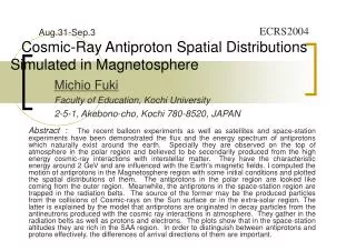
ICRC2003. OG.1.5.2. Calculation of Cosmic-Ray Proton and Anti-proton Spatial Distribution in Magnetosphere. Michio Fuki , Ayako Kuwahara, Nozomi, Sawada Faculty of Education, Kochi University JAPAN. Index. 1. INTRODUCTION Where/How much Anti-protons 2. METHOD (Models)

E N D
ICRC2003 OG.1.5.2 Calculation of Cosmic-Ray Proton and Anti-proton Spatial Distribution in Magnetosphere Michio Fuki, Ayako Kuwahara, Nozomi, Sawada Faculty of Education, Kochi University JAPAN
Index • 1. INTRODUCTION • Where/How much Anti-protons • 2. METHOD (Models) • Equation of Motion • Magnetic Fields • Injection Conditions • 3. RESULTS • Formation of Radiation Belts • Spatial Distributions • 4. CONCLUSIONS
1. INTRODUCTION • 1-1 Antiprotons and Magnetosphere • Balloon experiments (Anti-protons and Protons) • SPACE STATIONS (protons, electrons) • BESS, CAPRICE, etc. • AMS, HEAT, PAMERA… • Where/How much are Anti-protons around the Earth ? • Computer Simulation Study
2. METHOD (Model) 2-1 Equation of Motion Lorentz Force; V :velocity,m: mass , c : light velocity, B:Magnetic Field (static),q:electric charge, E = 0;No Electric Field
2-2 Magnetic Fields (static) • in case : Dipole Fields ….. Störmer theory • Rotation (spiral) • Bounce • Drift
IGRF (International Geomagnetic Reference Fields) • Spherical harmonic functions, 12th order • SAA region (low intensity) (South American Anomaly) • Inside Magnetosphere • Additional outer-belt components (Beard-Mead) in Magnetopause
2-3 Injection model Initial conditions • I) p (free protons from out of magnetosphere) Cosmic-ray proton • II) p + A → p + X (interaction with air) 20 km assumed , albedoproton • III)p + A → n + X n → p + e- + ν (decay from albedoneutron) τ = 900 sec, decayedproton Anti-protons are similar, but they are created. • III)p + A → p + n + n-+ X(pair-creation) n-→ p- + e+ + ν (decay from anti-neutron)
2-3 Injection model Initial conditions • I) p (free protons from out of magnetosphere) Cosmic-rays • II) p + A → p + X (interaction with air) 20 km assumed , albedo proton • III)p + A → n + X n → p + e- + ν (decay from albedo neutron) τ = 900 sec, decayed proton Anti-protons are similar, but they are created. • III)p + A → p + n + n-+ X (pair-creation) n-→ p- + e+ + ν (decay from anti-neutron)
2.4 Energy Spectra Fisk BESS Mode energy ~0.3 – 0.7 GeV Mode energy ~ 2.0 GeV
continue • Kinetic Energy Spectrum (Model-I&II) Em: mode energy, a, b: spectrum power index • Em =0.3 GeV for proton (solar quiet), • Em =2.0 GeV for anti-proton. • Index a = -1, b = 1.5. • For Model-III (decayed protons/anti-protons)
Calculation • 3-dimentional equations solved by time • Runge-Kutta-Gill method • Ranged from RE(=6,350km) to 10・RE • Time step sliced from 10 μsec to 10 msec • One particle traced maximum 10 minutes • Random Energy from 10 MeV to 10 GeV • Random starting points and directions • Random neutron decay by 900 sec (M-III)
3. RESULTS Trapping Probability • Three solutions • Escape …. Leave from the magnetosphere • Arrive …. Reach to the Earth • Trap …. Chaotic motion in magnetosphere (⇒ Van-Allen Radiation Belts) • Probabilities of three solutions from 3 models Typical @ 1 GeV (energy dependent)
Spatial Distribution (1) Model-II Model-I Model-III
continued Protons ~ 0.1 GeV, 1000 trials
Poles Surface distribution @400km ProtonModel-I 100000 events Anti-proton Model-I Poles diffused Spatial Distribution (2)
World Surface distribution ISS@400km ProtonModel-III 10000 particles Anti-proton Model-III SAA gathering continued
Height Distribution (Φ=-50,130deg) Protons・Antiprotons Spatial Distribution (3)
4. CONCLUSIONS • Cosmic-ray (anti-)protons apt to arrive in polar regions • Decayed protons trapped to form Van-Allen radiation belts (CRAND; cosmic-ray albedo neutron decay) • Lower energy protons well trapped due to life time • Higher energy Anti-protons may remain in radiation belts • Protons and anti-protons are gathered in SAA • Proton tails are east and anti-protons are west • Anti-protons center in altitude 2000km lower than protons • These are qualitative discussions
Closing • More statistics is necessary for quantitative discussions for absolute flux, p-/p ratio, energy spectra and direction distribution. • To compare with other theoretical results, simulation programs or coming experimental data.