Download
1 / 34
340 likes | 780 Vues
Multiple Regression and Regression Model Building. Woody Durham, commenting on a lopsided game between the Chicago Bulls and the New Jersey Nets (Dean Dome, 10/20/90): “Watching this game is as much fun as watching a multiple regression.”. A Comment on Regression.

E N D
Multiple Regression and Regression Model Building Multiple Regression
Woody Durham, commenting on a lopsided game between the Chicago Bulls and the New Jersey Nets (Dean Dome, 10/20/90): “Watching this game is as much fun as watching a multiple regression.” A Comment on Regression Multiple Regression
See the comparison in the coursepack on pp. 31-32 Multiple regression is a direct extension of simple regression Multiple Regression
Campus Stationery Store - the model which predicts sales using both advertising and price as independent variables - p. 27 We will let Excel do the calculations for us When using Excel, the independent variables need to be in neighboring columns Multiple regression example Multiple Regression
Often in business we use historical data to make forecasts about the future “Forecasting is like trying to drive a car blindfolded following directions given by a person who is looking out the back window.” Anonymous Using the multiple regression model for forecasting Multiple Regression
Two kinds of forecasting Point estimates - single, “best” guesses about the value of the dependent variable Interval estimates - a range of values in which the dependent variable is likely to occur Forecasting - the mechanics Multiple Regression
Just as with simple regression, we use the data to estimate the model parameters (the intercept and slope coefficients), and combine these with (given) values of the independent variables to forecast a value of the dependent variable Example - What level of sales would you predict for CSS when advertising level is 13 and price is 150? Multiple regression point estimates Multiple Regression
Just as with simple regression, we build an interval centered on the point estimate of y Approximate formulas for these interval estimates are on p. 32 of the coursepack Multiple regression interval estimates Multiple Regression
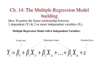
Testing the model itself A test for the overall model, i.e., testing the entire collection of independent variables for usefulness in predicting the dependent variable Tests for the usefulness of individual independent variables Statistical analyses with the multiple regression model Multiple Regression
This is a new test, i.e., one we did not discuss for simple regression (but it works there as well) There are three equivalent ways to express the hypotheses we will be testing Testing the overall model in multiple regression Multiple Regression
or or H0: The collection of x’s does not help to predict y Ha: The collection of x’s does help to predict y Testing the overall model, cont. Multiple Regression
The statistic we use to conduct these hypotheses tests is the F statistic in the ANOVA box of Excel’s Regression output Note in passing - the sampling distribution of this statistic is an F distribution. We will study this distribution later in the course Testing the overall model, cont. Multiple Regression
For the moment, the p-value for the test we want to conduct is the Significance F value in the Excel output Small Significance F values imply that the collection of independent variables does help to predict the dependent variable Testing the overall model, cont. Multiple Regression
Again we will be testing the following hypotheses: Testing the usefulness of individual x’s Multiple Regression
These tests will be conducted used Excel’s P-values contained in the bottom box of the Regression output As in simple regression Low p-value means the variable is useful in helping to predict y High p-value means the variable is not useful in helping to predict y Testing the individual x’s, cont. Multiple Regression
Strong relationships between the independent variables (Multicollinearity) Predicting outside the range of values of the independent variables Potential pitfalls of regression Multiple Regression
We will show how to generate and use two graphs The scatter diagram of the residuals vs. an independent variable The Normal probability plot of the residual values to check for three assumptions Constant scatter of the residuals (homoskedasticity) Linearity of the data Normality of the residuals Checking the assumptions Multiple Regression
All of these checks employ “art appreciation” Check for constant scatter and linearity using the scatter diagrams of the residuals vs. the independent variables In Excel, check the Residual Plots option in the Regression dialog box Checking the assumptions, cont. Multiple Regression
Constant scatter is not met if the residuals have different amounts of variation at different values of x - e.g., “butterfly” or “fan” shapes Linearity is not met if the residuals show a curved pattern as x varies Interpretation of the scatter diagrams Multiple Regression
Create the Normal probability plot of the residuals to check for Normality of the residuals To do this in Excel, follow the procedure given in the “Doing Regression Residual Analysis in Excel” section of the coursepack Checking the assumptions, cont. Multiple Regression
The residuals are Normally distributed if the points lie roughly in a straight-line pattern (along the reference line) The residuals are not Normally distributed if the points are curved relative to the reference line Interpretation of the Normal probability plot Multiple Regression
Basic idea - use a “dummy variable,” i.e., one that has only two values, 0 and 1 Example - exploration of potential salary bias in the “Illustrating Dummy Variables” section of the coursepack (you may have seen these data before!) Introducing qualitative variables into regression Multiple Regression
The original model if x2 is a dummy variable defined as If the salesperson is female If the salesperson is male Interpretation of the dummy variable model Multiple Regression
can be rewritten as which represents a pair of parallel models, with b2 representing the change for men relative towomen Forwomen For men Interpretation of the dummy variable model, cont.
Any dummy variable model has a “base” or “reference” case. (Determined by all the dummy variables = 0) All dummy variable coefficients are interpreted as changes relative to the base case Interpretation of the dummy variable model, cont. Multiple Regression
Key - add an interaction term to the model and b3 is the change in slope relative to the base case Building a model in which both slope and intercept change Multiple Regression
Create a dummy variable for each value of the qualitative variable Make sure you leave at least one of the dummy variables out of the model when you run it using Excel Example - the weight loss data analyzed in the “Qualitative / Quantitative Interactions” section of the packet Adding qualitative variables with more than two values Multiple Regression
Basic idea - compare “reduced” and “complete” models A statistical test to compare two regression models (Reduced) (Complete) Multiple Regression
Important - every variable in the reduced model must also be in the complete model Calculate the comparison statistic using numbers from both regression outputs Comparing two models, cont. Multiple Regression
A confusion - there are two ways to calculate the value of the statistic The book’s method Comparing two models, cont. Multiple Regression
And the method shown in the packet these will always give the same answer! Comparing two models, cont. Multiple Regression
This F statistic has an F sampling distribution with k - g, n-[k+1] d.f. The rejection region is in the upper-tail only Comparing two models, cont. Multiple Regression
If we use a polynomial model we can still estimate the parameters of the model using regression Fitting curved models to data Multiple Regression
In Excel, a column for each power of the values of the independent variable must be created Example - the chicken feed supplement problem in the “An Example of a One Variable, Second Order Model” in the coursepack Fitting curved models, cont. Multiple Regression