Download
1 / 25
250 likes | 360 Vues
Instrument modeling for High Contrast Imaging Tips and tools. Anthony Boccaletti Observatoire de Paris LESIA. Context. Several instruments dedicated to Exoplanet detection and characterization with High Contrast Imaging since 2001 For this decade : SPHERE and GPI : 2011/12

E N D
Instrument modeling for High Contrast ImagingTips and tools Anthony Boccaletti Observatoire de Paris LESIA
Context • Several instruments dedicated to Exoplanet detection and characterization with High Contrast Imaging since 2001 • For this decade : • SPHERE and GPI : 2011/12 • JWST-MIRI : 2015 • For the future (>2020-25): • ELT / EPICS • Space coronagraphs : ACCESS, PECO, SPICES …. => need for simulation tools adapted to the instruments and to the observing cases
Favorite Techniques Issues or noises related to Image formation (so to the source itself)
Many other sources of noise • Background : sky, thermal emission of instrument/telescope, zodiacal light, exozodi • Detector related : Flat Field, readout noise, remanance, … • Many others that we don't even thought about !!!
Interest of instrument modeling • Assess the performance for a science case • Evaluate the limitations : which source of noise, or which issues are relevant ? • Put some constraints on the instrument design • Optimize the design itself (instrumental choices) • And then => reassess the performance
Generic concept of a coronagraph pupille plan focal + diaphragme détecteur + masque pupille FFT-1 FFT FFT Plan C Plan D Plan A Plan B
The mathematical formulation Plan A: si Plan B: Plan C: Plan D:
A good example : SPHERE High frequency AO correction (41x41 act.) High stability : image / pupil control Visible – NIR Refraction correction FoV = 12.5’’ 40x40 SH-WFS in visible 1.2 KHz, RON < 1e- Beam control (DM, TT, PTT, derotation) Pola control Calibration Coronagraphic imaging: Dual polarimetry, direct BB + NB. λ = 0.5 – 0.9 µm, λ/2D @ 0.6 µm, FoV = 3.5” 0.95 – 1.35/1.65 µm λ/2D @ 0.95 µm, Spectral resolution: R = 54 / 33 FoV = 1.77” Pupil apodisation, Focal masks: Lyot, A4Q, ALC. IR-TT sensor for fine entering 0.95 – 2.32 µm; λ/2D @ 0.95 µm Differential imaging: 2 wavelengths, R~30, FoV = 12.5’’ Long Slit spectro: R~50 & 400 Differential polarization Nasmyth platform, static bench, Temperature control, cleanliness control Active vibration control
Context and Issues Calibration of the residual speckle pattern is needed • characterization of Giant Planets and Brown Dwarves : contrast of 10-6 / 10-7 @ 0.5’’ • instrumentation : - exAO • - coronography contrast ~ 6.10-5
Speckle calibration is needed différentiel pupille plan focal + diaphragme détecteur + masque pupille FFT-1 FFT FFT Plan C Plan D Plan A Plan B
Spectral Differential Imaging filter 1 detector telescope AO coronagraph filter 2 data are rescaled and normalized in intensity - single subtraction : obj() – obj() - spectral obj() – ref() - temporal (reference star or filters swapping) - double subtraction : [obj() – obj()] – [ref() – ref()] calibration of common aberrations (dynamic & static) calibration of differential aberrations (static)
In more details AO filtering phase diversity filtering • phase & amplitude screen, (atmospheric): , , star, ref • instrumental jitter • telescope aberrations • aberrations: telescope -> dichroïc • aberrations: dichroic -> corono pupil plane 1 FFT • pupil shear: (, , star, ref) • pointing: (, , star, ref) focal plane 1 (coro. mask) - corono (4Q, achro 4Q, Lyot, apo Lyot): chromatism FFT-1 pupil plane 2 (Lyot stop) - common aberrations corono -> detector - differential aberrations corono -> detector (, ) FFT • Lyot stop shear (star, ref) • flux normalisation: star, ref, planets (, ) • background • RON • flat field (, , star, ref) • single subtraction • double subtraction • detectivity plot focal plane 2
Some tips to begin with … • Sampling of the pupil : • good sampling needed to reproduce pupil shape • Make use of grey approx. • Sampling of the image • PSF size = N / D = lambda/D (N: array size, D: pupil diameter) • PSF chromaticity • Modify pupil size but keep the array constant => change the actual shape of the pupil • Modify array size but keep the pupil constant • Uses of FFT with IDL • Shift the center to coordinates [0,0] • Aliasing: make sure N is at least 2xD
Some tips to begin with … • Image normalization: • use an off-axis object far from the center (not affected by the mask) but account for the throughput • Wavefront errors: • Define the Power Spectrum Density of aberrations with power law and cut-off frequencies • WFE screen = random screen X sqrt (PSD)
The exercise • Produce coronagraphic images at two simultaneous wavelengths for a star and a reference target. Compare contrast curves (5s) at different stages: coronagraphic image, 2-l subtraction, ref-subtraction, double subtraction
The exercise: guidelines • 2 codes : 1 for image formation and 1 for contrast curves • Image formation • Make pupil • generate common aberrations + differential temporal aberrations upstream • Build complex amplitude in pupil • Build PSF complex amplitude • Make coronagraphic image for on-axis and off-axis objects • Save results • Contrast curves • Read results • Normalize • Resample l1 to l0 • Calculate various subtraction • Plot contrast curves
The exercise: guidelines • Image formation • Start with circular pupil then use the routine sph_pupil to produce VLT pupil in grey level. • Generate diaphragm (under/over-sized) • Define bands: H2 H3 filters of SPHERE = 1.593 & 1.667 microns • upstream aberrations : • use the provided VLT_wfe.fits • Add a 4nm defocus on the reference target • Define a loop on filter and scale array size accordingly • Calculate complex amplitude in pupil : sph_amp_complex.pro • Build PSFs with sph_psf.pro • Introduce differential aberrations with sph_wfdiff.pro • Build coronagraphic images with sph_corono.pro • Take intensities • Rescale the arrays to 1kx1k with sph_taille.pro • Produce off-axis planets with sph_planet.pro • Save results
The exercise: guidelines • Contrast curves: • Read results of image formation • Resample to camera pixels (shannon at 0.95mic) make use of sph_rescale.pro • Resample of image at l1 to l0 (again sph_rescale.pro) • Calculate subtractions: • obj(l0)-ref(l0) • obj(l0)-obj(l1) • [obj(l0)-obj(l1)] – [ref(l0)-ref(l1)] • Azimuthal contours with sph_profil1d.pro • Plot averaged contour for psf and corono image and 5sig level for subtractions
The exercise: guidelines • And play with the parameters …. • D = 8m / 160 pix • N = 1024 • 40 linear actuators • Relative offset (star/ref) = 0.5 mas • Differential aberrations = 10nm • Planet separations = 0.1", 0.5", 1"
More tools … • Reference to : • CAOS + SPHERE Software package (public) • PROPER by John Krist (public) • PESCA for ELT (not public)