Download
1 / 152
2.25k likes | 3.46k Vues
CHAPTER 2. First-Order Differential Equations. Chapter Contents. 2.1 Solution Curves Without a Solution 2.2 Separable Variables 2.3 Linear Equations 2.4 Exact Equations 2.5 Solutions by Substitutions 2.6 A Numerical Methods 2.7 Linear Models 2.8 Nonlinear Model

E N D
CHAPTER 2 First-Order Differential Equations
Chapter Contents • 2.1 Solution Curves Without a Solution • 2.2 Separable Variables • 2.3 Linear Equations • 2.4 Exact Equations • 2.5 Solutions by Substitutions • 2.6 A Numerical Methods • 2.7 Linear Models • 2.8 Nonlinear Model • 2.9 Modeling with Systems of First-Order DEs
2.1 Solution Curve Without a Solution • IntroductionBegin our study of first-order DE with analyzing a DE qualitatively. • SlopeA derivative dy/dx of y = y(x)gives slopes of tangent lines at points. • Lineal ElementAssume dy/dx = f(x, y(x)). The value f(x, y) represents the slope of a line, or a line element is called a lineal element. See Fig 2.1.1.
Fig 2.1.1 Solution curve is tangent to linear element at (2, 3)
Direction Field • If we evaluate f over a rectangular grid of points, and draw a lineal element at each point (x, y) of the grid with slope f(x, y), then the collection is called a direction fieldor a slope field of the following DEdy/dx = f(x, y)
Example 1 Direction Field • The direction field of dy/dx = 0.2xy is shown in Fig 2.1.2(a) and for comparison with Fig 2.1.2(a), some representative graphs of this family are shown in Fig 2.1.2(b).
Example 2 Direction Field Use a direction field to draw an approximate solution curve for dy/dx = sin y, y(0) = −3/2. Solution:Recall from the continuity of f(x, y) and f/y = cos y. Theorem 1.2.1 guarantees the existence of a unique solution curve passing any specified points in the plane. Now split the region containing (-3/2, 0) into grids. We calculate the lineal element of each grid to obtain Fig 2.1.3.
Increasing/DecreasingIf dy/dx > 0 for all x in I, then y(x) is increasing in I.If dy/dx < 0 for all x in I, then y(x) is decreasing in I. • DEs Free of the Independent variable dy/dx = f(y)(1)is called autonomous. We shall assume f and f are continuous on some I.
Critical Points • The zeros of f in (1) are important. If f(c) = 0, then c is a critical point, equilibrium point or stationary point. • Substitute y(x) = c into (1), then we have 0 = f(c) = 0. • If c is a critical point, then y(x) = c, is a solution of (1). • A constant solution y(x) = c of (1) is called an equilibrium solution.
Example 3 An Autonomous DE The following DE dP/dt = P(a – bP)where a and b are positive constants, is autonomous.From f(P) = P(a – bP)= 0,the equilibrium solutions are P(t) = 0 and P(t) = a/b. Put the critical points on a vertical line. The arrows in Fig 2.1.4 indicate the algebraic sign of f(P) = P(a – bP). If the sign is positive or negative, then P is increasing or decreasing on that interval.
Solution Curves • If we guarantee the existence and uniqueness of (1), through any point (x0, y0) in R, there is only one solution curve. See Fig 2.1.5(a). • Suppose (1) possesses exactly two critical points, c1, and c2, where c1< c2. The graph of the equilibrium solution y(x) = c1, y(x) = c2 are horizontal lines and split R into three regions, say R1, R2and R3as in Fig 2.1.5(b).
Fig 2.1.5 Lines y(x)=c1 and y(x)=c2 partition R into three horizontal subregions
Some discussions without proof: (1) If (x0, y0) in Ri, i = 1, 2, 3,when y(x)passes through (x0, y0),will remain in the same subregion. See Fig 2.1.5(b). (2) By continuity of f, f(y)can not change signs in a subregion. (3) Since dy/dx = f(y(x)) is either positive or negative in Ri, a solution y(x) is monotonic.
(4)If y(x) is bounded above by c1, (y(x) < c1), the graph of y(x) will approach y(x) = c1;If c1 < y(x) < c2,it will approach y(x) = c1and y(x) = c2;If c2 < y(x), it will approach y(x) = c2;
Example 4 Example 3 Revisited Referring to example 3, P =0and P = a/b are two critical points, so we have three intervals for P:R1: (-, 0),R2 : (0, a/b),R3 : (a/b, )Let P(0) = P0and when a solution pass through P0,wehave three kind of graph according to the interval where P0 lies on. See Fig 2.1.6.
Fig 2.1.6 Phase portrait and solution curve in each of the three subregions in Ex 4
Example 5 Solution Curves of an Autonomous DE The DE: dy/dx = (y – 1)2possesses the single critical point 1. From Fig 2.1.7(a), we conclude a solution y(x) is increasing in - < y < 1 and 1 < y < , where - < x < . See Fig 2.1.7.
Attractors and Repellers • See Fig 2.1.8(a). When y0 lies on either side of c, it will approach c. This kind of critical point is said to be asymptotically stable, also called an attractor. • See Fig 2.1.8(b). When y0 lies on either side of c, it will move away from c. This kind of critical point is said to beunstable, also called a repeller. • See Fig 2.1.8(c) and (d). When y0 lies on one side of c, it will be attracted to c and repelled from the other side.This kind of critical point is said to be semi-stable.
Fig 2.1.8 Critical point c is an attractor in (a), a repeller in (b), and semi-stable in (c) and (d)
Autonomous DEs and Direction Fields • Fig 2.1.9 shows the direction field of dy/dx = 2y – 2.It can be seen that lineal elements passing through points on any horizontal line must have the same slope. Since the DE has the form dy/dx = f(y),the slope depends only on y.
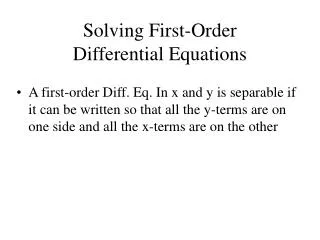
Definition 2.2.1 Separable Equations A first-order DE of the formdy/dx = g(x)h(y)is said to be separable or to have separable variables. 2.2 Separable Variables • Introduction: Consider dy/dx = f(x, y) = g(x).The DEdy/dx = g(x)(1)can be solved by integration. Integrating both sides to get y = g(x) dx = G(x) + c.eg: dy/dx = 1 + e2x, then y = (1 + e2x)dx = x + ½ e2x + c
Rewrite the above equation as(2)where p(y) =1/h(y).When h(y) = 1, (2) reduces to (1).
If y = (x)is a solution of (2), we must have and(3)But dy = (x) dx, (3)is the same as(4)
Example 1 Solving a Separable DE Solve (1 + x) dy – y dx = 0. Solution:Since dy/y = dx/(1 + x), we haveReplacing by c, gives y = c(1 + x).
Example 2 Solvong Curve Solve Solution:We also can rewrite the solution asx2+ y2 = c2,where c2 =2c1Apply the initial condition, 16 + 9 = 25 = c2See Fig 2.2.1.
Losing a Solution • When r is a zero of h(y), then y = r is also a solution of dy/dx = g(x)h(y).However, this solution will not show up after integration. That is a singular solution.
Example 3 Losing a Solution Solve dy/dx = y2 – 4. Solution:Rewrite this DE as(5)then
Example 3 (2) Replacing by c andsolving for y, we have(6)If we rewrite the DE as dy/dx = (y + 2)(y – 2),from the previous discussion, we have y = 2is a singular solution.
Example 4 An Initial-Value Problem Solve Solution:Rewrite this DE asusing sin2x = 2sin x cos x, then (ey – ye-y) dy = 2sin x dx from integration by parts,ey + ye-y + e-y = -2cos x + c (7)From y(0) =0,we have c = 4 to getey + ye-y + e-y = 4 −2 cos x (8)
Use of Computers • Let G(x, y) = ey + ye-y + e-y + 2cos x. Using some computer software, we plot the level curves of G(x, y) = c. The resulting graphs are shown in Fig 2.2.2 and Fig 2.2.3.
Fig 2.2.2 Level curves G(x, y)=c, where G(x, y) = ey + ye-y + e-y + 2cos x
If we solve dy/dx = xy½, y(0) = 0(9)The resulting graphs are shown in Fig 2.2.4.
Definition 2.3.1 Linear Equations A first-order DE of the forma1(x)(dy/dx) + a0(x)y = g(x)(1)is said to be a linear equationiny. 2.3 Linear Equations • IntroductionLinear DEs are friendly to be solved. We can find some smooth methods to deal with. • When g(x) = 0,(1) is said to be homogeneous; otherwise it is nonhomogeneous.
Standard FormThe standard for of a first-order DE can be written asdy/dx + P(x)y = f(x)(2) • The PropertyDE (2) has the property that its solution is sum of two solutions, y = yc + yp, where yc is a solution of the homogeneous equationdy/dx + P(x)y = 0(3)and yp is a particularsolution of (2).
VerificationNow (3) is also separable. Rewrite (3) as • Solving for y gives
Variation of Parameters • Let yp = u(x) y1(x), where y1(x)is defined as above.We want to find u(x) so that yp is also a solution. Substituting ypinto (2) gives
Since dy1/dx + P(x)y1 = 0, so that y1(du/dx) = f(x) Rearrange the above equation, From the definition of y1(x), we have(4)
Solving Procedures • If (4) is multiplied by(5)then(6)is differentiated(7)we get(8)Dividing (8) by gives (2).
Guidelines for Solving a Linear First-Order Equation Put a linear equation of form (1) into standard form (2) and then determine P(x) and the integrating factor Multiply (2) by the integration factor. The left side of the resulting equation is automatically the derivative of the integrating factor and y. Writeand then integrate both sides of this equation. Integrating Factor • We call y1(x) = is an integrating factorand we should only memorize this to solve problems.
Example 1 Solving a Linear DE Solve dy/dx – 3y = 6. Solution:Since P(x)= – 3,we have the integrating factor is then is the same as So e-3xy = -2e-3x + c, a solution is y = -2 + ce3x, - < x < .
Notes • The DE of example 1 can be written as so that y = –2is a critical point.
General Solutions • Equation (4) is called the general solution on some interval I. Suppose again P and f are continuous on I. Writing (2) as Suppose again Pandfare continuous onI. Writing (2)as y = F(x, y)we identify F(x, y) = – P(x)y + f(x),F/y = –P(x)which are continuous on I.Then we can conclude that there exists one and only one solution of(9)
Example 2 General Solution Solve Solution:Dividing both sides by x, we have(10)So, P(x)= –4/x, f(x) = x5ex, P and f are continuous on (0, ).Since x > 0,we write the integrating factor as