Download
1 / 18
180 likes | 359 Vues
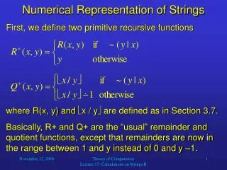
Numerical Representation of Strings. First, we define two primitive recursive functions. where R(x, y) and x / y are defined as in Section 3.7.

E N D
Numerical Representation of Strings First, we define two primitive recursive functions where R(x, y) and x / y are defined as in Section 3.7. Basically, R+ and Q+ are the “usual” remainder and quotient functions, except that remainders are now in the range between 1 and y instead of 0 and y –1. Theory of Computation Lecture 17: Calculations on Strings II
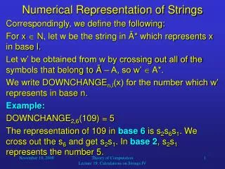
Numerical Representation of Strings So whenever y divides x, we do not have a remainder of 0 but a remainder of y, and accordingly the quotient is one number below the “actual” quotient. Therefore, like with the usual quotient and remainder, it is still true that: x/y = Q+(x, y) + R+(x, y)/y, only that now we have 1 R+(x, y) y. We will use the functions Q+ and R+ to show how to obtain the subscripts i0, i1, …, ik from any integer x > 0. Theory of Computation Lecture 17: Calculations on Strings II
Numerical Representation of Strings Let us define: u0 = x um+1 = Q+(um, n) Then we have: u0 = iknk + ik-1nk-1 + … + i1n1 + i0 u1 = iknk-1 + ik-1nk-2 + … + i1 : uk = ik The “remainders” R+ are exactly the values of the im: im = R+(um, n), m = 0, …, k. Theory of Computation Lecture 17: Calculations on Strings II
Numerical Representation of Strings This is analogous to our usual base-n notation: u0 = x um+1 = Q(um, n) Then we have: u0 = iknk + ik-1nk-1 + … + i1n1 + i0 u1 = iknk-1 + ik-1nk-2 + … + i1 : uk = ik The remainders R are exactly the values of the im: im = R(um, n), m = 0, …, k. Theory of Computation Lecture 17: Calculations on Strings II
Numerical Representation of Strings Example: Find binary representation of number 13: Then u0 = x = 13; n = 2 u1 = Q(13, 2) = 6; i0 = R(13, 2) = 1 u2 = Q(6, 2) = 3; i1 = R(6, 2) = 0 u3 = Q(3, 2) = 1; i2 = R(3, 2) = 1 u4 = Q(1, 2) = 0; i3 = R(1, 2) = 1 Then w = 1101. Thus k = 3 and we have x = 123 + 122 + 021 + 120 Theory of Computation Lecture 17: Calculations on Strings II
Numerical Representation of Strings You certainly noticed that in our string representation we used symbols s1, …, sn, while in the everyday number representation we use s0, …, sn-1. So what exactly are the analogies and differences between the two systems? To find out about this, let us look at the following modified set of digits D: D = {s1, …, s10} = {1, 2, 3, 4, 5, 6, 7, 8, 9, X} Here, the X stands for a digit with the value 10, while there is no digit with the value 0. Theory of Computation Lecture 17: Calculations on Strings II
Numerical Representation of Strings So what is the number x associated with the stringw = 76 ? x = 710 + 6 = 76 And what is the number for w = 3X6 ? x = 3100 + 1010 + 6 = 406 Finally, what is the number for w = XX ? x = 1010 + 10 = 110 These examples already suggest that we can use this system in a way quite similar to our “usual” system. Theory of Computation Lecture 17: Calculations on Strings II
Numerical Representation of Strings Now let us turn this around: What is the string w associated with the number x = 39? w = 39 (as long as x does not contain any 0s, w is the “usual” decimal string representing x) And what is the string for x = 100 ? w = 9X But what is the string for x = 504 ? w = 4X4 Finally, what is the string for x = 0 ? w = 0 (0 is the null string symbol) Theory of Computation Lecture 17: Calculations on Strings II
Numerical Representation of Strings We can even transfer our elementary arithmetic to the new system: X 4 + 5 9 6 1 0 4 corresponding to + 5 9 6 7 0 0 6 9 X X 2 3 - X 1X 1 0 2 3 corresponding to - 1 0 2 0 3 3 Theory of Computation Lecture 17: Calculations on Strings II
Numerical Representation of Strings This applies even to multiplication: 3 X X 7 4 0 corresponding to 1 0 7 4 2 8 0 2 7 X 3 9 X 7 4 2 X Theory of Computation Lecture 17: Calculations on Strings II
Numerical Representation of Strings So you see that we can easily replace our usual digit range from 0 to n-1 with the range 1 to n. In our representation of strings on the alphabet A, we use the range from 1 to n to have a bijective mapping between strings and numbers. When using a range from 0 to n-1, there is no such mapping, because different strings correspond to the same number, for example: 87 = 087 = 0087 = 00087 = … Theory of Computation Lecture 17: Calculations on Strings II
Numerical Representation of Strings Now let us return to our general case of associating numbers with strings. For an alphabet A = {s1, …, sn}, the stringw = siksik-1… si1, si0is called the base n notation for the number x as defined by x = iknk + ik-1nk-1 + … + i1n1 + i0 . When n is fixed, we can consider a function of one or more variables on A* as a function of the corresponding numbers. Theory of Computation Lecture 17: Calculations on Strings II
Numerical Representation of Strings So we can speak of an m-ary partial function on A* with values in A* as being partially computable, or when it is total, we can speak of it as being computable. Similarly, we can say that an m-ary function on A* is primitive recursive. But what about predicates? Notice that for an alphabet A = {s1, …, sn} the value s1 denotes 1 in base n notation. Thus an m-ary predicate on A* is simply a total m-ary function on A* whose values are either s1 (“true”) or 0 (“false”). Therefore, it makes sense to speak of an m-ary predicate on A* as being computable. Theory of Computation Lecture 17: Calculations on Strings II
Numerical Representation of Strings For a given alphabet A, any subset of A* (any set of strings on A) is called a language on A. By associating numbers with the elements of A*, we can speak of a language on A as being r.e., recursive, or primitive recursive. Notice that our base n notation even works for n = 1, that is, an alphabet containing only one symbol. For example, if A = {s1} then x = 1 is represented by the string w = s1 x = 7 is represented by the string w = s1s1s1s1s1s1s1 : Theory of Computation Lecture 17: Calculations on Strings II
Numerical Representation of Strings To avoid confusion, we will not use decimal digits as symbols in our alphabets. Accordingly, a string of decimal digits will always be meant to refer to a number. We will now define some useful functions for string operations. The first function will be CONCAT. Theory of Computation Lecture 17: Calculations on Strings II
Numerical Representation of Strings Let A be some fixed alphabet containing n symbols, A = {s1, …, sn}. For each m 1, we define CONCATn(m) as follows: CONCATn(1)(u) = u CONCATn(m+1)(u1, …, um, um+1) = zum+1, where z = CONCATn(m)(u1, …, um). This means that for given strings u1, …, um A*, CONCATn(m)(u1, …, um) is obtained by concatenating the strings u1, …, um. Theory of Computation Lecture 17: Calculations on Strings II
Numerical Representation of Strings We will usually omit the superscript, i.e., the number of arguments. For example: CONCAT3(s3s1s2, s1s3) = s3s1s2s1s3 Translating this equation from strings to numbers: CONCAT3(32, 6) = 294 It is also true that CONCAT5(s3s1s2, s1s3) = s3s1s2s1s3 Translating this equation from strings to numbers: CONCAT5(82, 8) = 2058 Obviously, the definition of CONCAT depends on the base n. Theory of Computation Lecture 17: Calculations on Strings II
Numerical Representation of Strings We will now look at several primitive recursive functions on strings. These functions will be useful for our further discussion of calculation on strings. It will be helpful to remember the functions g and h: g(0, n, x) = x g(m + 1, n, x) = Q+(g(m, n, x), n), then g(m, n, x) = um. h(m, n, x) = R+(g(m, n, x), n), then im = h(m, n, x), m = 0, …, k. Theory of Computation Lecture 17: Calculations on Strings II