Download
1 / 31
310 likes | 515 Vues
SIO 210: Dynamics I Momentum balance (no rotation) L. Talley Oct. 13, 2010. Continuity (mass conservation) Reading: DPO ch. 5.1 Stewart chapter 7.7 (more formal) Force balance Reading: DPO ch. 7.1, 7.2 (skip 7.2.3) Lecture emphasis: advection, pressure gradient force

E N D
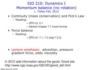
SIO 210: Dynamics IMomentum balance (no rotation)L. Talley Oct. 13, 2010 • Continuity (mass conservation) • Reading: • DPO ch. 5.1 • Stewart chapter 7.7 (more formal) • Force balance • Reading: • DPO ch. 7.1, 7.2 (skip 7.2.3) • Lecture emphasis: advection, pressure gradient force • Diffusivity to be covered by J. MacKinnon on Oct. 15
Equations for fluid mechanics • Mass conservation (continuity) (no holes) (covered in previous lecture) • Force balance: Newton’s Law ( ) (3 equations) • Equation of state (for oceanography, dependence of density on temperature, salinity and pressure) (1 equation) • Equations for temperature and salinity change in terms of external forcing, or alternatively an equation for density change in terms of external forcing (2 equations) • 7 equations to govern it all
Completed force balance (no rotation) (preview of coming attractions) acceleration + advection = pressure gradient force + viscous term x: u/t + u u/x + v u/y + w u/z = - (1/)p/x + /x(AHu/x) + /y(AHu/y) +/z(AVu/z) y: v/t + u v/x + v v/y + w v/z = - (1/)p/y + /x(AHv/x) + /y(AHv/y) +/z(AVv/z) z: w/t + u w/x + v w/y + w w/z = - (1/)p/z - g + /x(AHw/x) + /y(AHw/y) +/z(AVw/z)
Preliminaries: coordinate systems • In this course we use Cartesian coordinates • For problems on the Earth surface, these are “local” coordinates, with (0,0,0) at local center of problem. • East = x with velocity u • North = y with velocity v • Vertical = z with velocity w (0 at sea surface) • For much larger scales, we use spherical coordinates. (Not in this course.) (Geophysicists are even more careful and use oblate spheroidal coordinates since Earth is slightly oblate.)
Continuity (mass conservation) (review from previous lecture) The in and out arrows can be through any face of the box. For Mass Conservation, also include density at each face (mass transport) • DPO Fig. 5.2
Force balance • Newton’s law F = ma (from physics class) This is a vector equation, with 3 equations for each of the three directions (x, y and z) ma = F (for fluids) Divide by volume, so express in terms of density and force per unit volume : a = “Acceleration” in a fluid has two terms: actual acceleration and advection
Time change and Acceleration • Time change the change in stuff with time, for instance temperature T: T/t = T/t (Units are stuff/sec; here heat/sec or J/sec or W) • Acceleration: the change in velocity with time u/t = u/t (Units are velocity/sec, hence m/sec2) DPO Fig. 7.1
Advection • Move “stuff” - temperature, salinity, oxygen, momentum, etc. • By moving stuff, we might change the value of the stuff at the next location. We only change the value though if there is a difference (“gradient”) in the stuff from one point to the next • Advection is proportional to velocity and in the same direction as the velocity • E.g. u T/x or u T/xis the advection of temperature in the x-direction • Effect on time change of the property: T/t = -u T/x DPO Fig. 7.1
Forces acting on geophysical fluid • Gravity: g = 9.8 m/sec2 • Pressure gradient force • Friction (dissipation) (viscous force) DPO Fig. 7.1
Forces acting on geophysical fluid • Gravity: g = 9.8 m/sec2 • Pressure gradient force • Friction (dissipation) (viscous force) Towards center of Earth DPO Fig. 7.1
Forces acting on geophysical fluid • Gravity • Pressure gradient force • Friction (dissipation) (viscous force) DPO Fig. 7.1
Forces acting on geophysical fluid: vertical force balance • Gravity: g = 9.8 m/sec2 • Pressure gradient force • Friction (dissipation) (viscous force) Vertical balance: Vertical acceleration +advection = pressure gradient force + gravity + viscous Hydrostatic balance: Dominant terms for many phenomena – “static” – very small acceleration and advection Viscous term is very small 0 = PGF + gravity (in words) 0 = -p/z - g (equation) Towards center of Earth
Example of pressure gradientsDaily surface pressure map (in the atmosphere, we can simply measure the pressure at the surface)
Horizontal pressure gradient force • Small deviations of sea surface drive all flows - usually much less than 1 meter height. Pressure gradient is very difficult to measure directly. Gulf Stream example 1 meter height Equivalent to pressure of 1 dbar, since water density is ~ 1000 kg/m3 1 meter height 100 kilometers width (rest of water column: 5 km deep) LOW HIGH Pressure gradient is directed from low to high. Calculate size. Pressure gradient force is directed from high to low (water pushed towards lower pressure).
Compute acceleration due to PGF • Take the example of the Gulf Stream and compute the velocity after 1 year of acceleration. • (To calculate this, note that the PGF is -(1/)p/x and that the pressure difference is given from the hydrostatic balance -(1/)p/z = g; use g=9.8 m/s2, z=1 m; x = 100 km. Then u/t for acceleration, t = 1 year ~ 3.14x10⁷ sec.) • You’ll find it’s ridiculously large (compared with the observed 1 m/sec). How is such a large pressure gradient maintained without large velocities? • (answer: Earth’s rotation - Coriolis to be discussed later)
Mixing and diffusion • Random motion of molecules carries “stuff” around • Fick’s Law: net flux of “stuff” is proportional to its gradient • Flux = -(Qa-Qb)/(xa-xb) = -Q • where is the diffusivity Units: [Flux] = [velocity][stuff], so [] = [velocity][stuff][L]/[stuff] = [L2/time] = m2/sec
Flux Mixing and diffusion Fick’s Law: flux of “stuff” is proportional to its gradient Flux = -Q • If the concentration is exactly linear, with the amount of stuff at both ends maintained at an exact amount, then the flux of stuff is the same at every point between the ends, and there is no change in concentration of stuff at any point in between. Qb at xb Concentration Q(x) Qa at xa
Buildup of Q here due to convergence of flux Mixing and diffusion Diffusion: if there is a convergence or divergence of flux then the “stuff” concentration can change xb Flux Concentration Q(x) Removal of Q here due to divergence of flux xa
Diffusion term Buildup of Q here due to convergence of flux Mixing and diffusion Change in Q with time = Q/t = change in Q flux with space = -Flux/x = Q/t = 2Q/x2 xb Flux Concentration Q(x) Removal of Q here due to divergence of flux xa
Viscosity • Viscosity: apply same Fick’s Law concept to velocity. So viscosity affects flow if there is a convergence of flux of momentum. • Stress (“flux of momentum”) on flow is (= “flux”) = -u where is the viscosity coefficient DPO Fig. 7.3
Acceleration due to viscosity DPO Fig. 7.1
Acceleration due to viscosity • u/t = 2u/x2 = 2u/x2 [Fine print: is the kinematic viscosity and is the absolute (dynamic) viscosity) If the viscosity itself depends on space, then it of course needs to be INSIDE the space derivative: x(u/x) ]
Eddy diffusivity and eddy viscosity (to be expanded by J. MacKinnon,next lecture) • Molecular viscosity and diffusivity are extremely small (values given on later slide) • We know from observations that the ocean behaves as if diffusivity and viscosity are much larger than molecular (I.e. ocean is much more diffusive than this) • The ocean has lots of turbulent motion (like any fluid) • Turbulence acts on larger scales of motion like a viscosity - think of each random eddy or packet of waves acting like a randomly moving molecule carrying its property/mean velocity/information
Eddy diffusivity and viscosity Gulf Stream (top) and Kuroshio (bottom): meanders and makes rings (closed eddies) that transport properties to a new location
Eddy diffusivity and viscosity Example of surface drifter tracks: dominated to the eye by variability (they can be averaged to make a very useful mean circulation)
Measurements of mixing in ocean: horizontal and vertical diffusion are very different from each other and much larger than molecular diffusion • Intentional dye release, then track the dye over months Ledwell et al Nature (1993) Horizontal diffusion Vertical diffusion
Values of molecular and eddy diffusivity and viscosity • Molecular diffusivity and viscosity T = 0.0014 cm2/sec (temperature) S = 0.000013 cm2/sec (salinity) = 0.018 cm2/sec at 0°C (0.010 at 20°C) • Eddy diffusivity and viscosity values for heat, salt, properties are the same size (same eddies carry momentum as carry heat and salt, etc) But eddy diffusivities and viscosities differ in the horizontal and vertical • Eddy diffusivity and viscosity AH = 104 to 108 cm2/sec (horizontal) = 1 to 104 m2/sec AV = 0.1 to 1 cm2/sec (vertical) = 10-5 to 10-4 m2/sec
Completed force balance (no rotation) Three equations: Horizontal (x) (west-east) acceleration + advection = pressure gradient force + viscous term Horizontal (y) (south-north) acceleration + advection = pressure gradient force + viscous term Vertical (z) (down-up) acceleration +advection = pressure gradient force + gravity + viscous term
Completed force balance (no rotation) acceleration + advection = pressure gradient force + viscous term x: u/t + u u/x + v u/y + w u/z = - (1/)p/x + /x(AHu/x) + /y(AHu/y) +/z(AVu/z) y: v/t + u v/x + v v/y + w v/z = - (1/)p/y + /x(AHv/x) + /y(AHv/y) +/z(AVv/z) z: w/t + u w/x + v w/y + w w/z = - (1/)p/z - g + /x(AHw/x) + /y(AHw/y) +/z(AVw/z)
Some scaling arguments • Full set of equations governs all scales of motion. How do we simplify? • We can use the size of the terms to figure out something about time and length scales, then determine relative size of terms, then find the approximate force balance for the specific motion. • Introduce a non-dimensional term that helps us decide if the viscous terms are important Acceleration Advection …… Viscosity U/TU2/L …… U/L2 Reynolds number: Re = UL/ is the ratio of advective to viscous terms Large Reynolds number: flow nearly inviscid (quite turbulent) Small Reynolds number: flow viscous (nearly laminar)
Equations for temperature, salinity, density • Temperature is changed by advection, heating, cooling, mixing (diffusion and double diffusion) • Salinity is changed by advection, evaporation, precipitation/runoff, brine rejection during ice formation, mixing (diffusion and double diffusion) • Density is related to temperature and salinity through the equation of state. • Often we just write an equation for density change and ignore separate temperature, salinity