Download
1 / 116
1.17k likes | 1.38k Vues
Data Minin g and Knowledge Acquizition — Chapter 2 — — Data Preprocessing —. 2013/2014 Summer. Chapter 2: Data Preprocessing. Why preprocess the data? Descriptive data summarization Data cleaning Data integration and transformation Data reduction

E N D
Data Mining and Knowledge Acquizition — Chapter 2 —— Data Preprocessing — 2013/2014 Summer
Chapter 2: Data Preprocessing • Why preprocess the data? • Descriptive data summarization • Data cleaning • Data integration and transformation • Data reduction • Discretization and concept hierarchy generation • Summary
Mining Data Dispersion Characteristics • Motivation • To better understand the data: central tendency, variation and spread • Data dispersion characteristics • median, max, min, quantiles, outliers, variance, etc. • Numerical dimensions correspond to sorted intervals • Data dispersion: analyzed with multiple granularities of precision • Boxplot or quantile analysis on sorted intervals • Dispersion analysis on computed measures • Folding measures into numerical dimensions • Boxplot or quantile analysis on the transformed cube
Measuring the Central Tendency • Mean (algebraic measure): • Weighted arithmetic mean: • Trimmed mean: chopping extreme values • Median: A holistic measure • Middle value if odd number of values, or average of the middle two values otherwise • Estimated by interpolation (for grouped data) • Mode • Value that occurs most frequently in the data • Unimodal, bimodal, trimodal • Empirical formula:
Symmetric vs. Skewed Data • Median, mean and mode of symmetric, positively and negatively skewed data
Measuring the Dispersion of Data • Quartiles, outliers and boxplots • Quartiles: Q1 (25th percentile), Q3 (75th percentile) • Inter-quartile range: IQR = Q3 –Q1 • Five number summary: min, Q1, M,Q3, max • Boxplot: ends of the box are the quartiles, median is marked, whiskers, and plot outlier individually • Outlier: usually, a value higher/lower than 1.5 x IQR • Variance and standard deviation • Variance s2: (algebraic, scalable computation) • Standard deviation s is the square root of variance s2
Properties of Normal Distribution Curve • The normal (distribution) curve • From μ–σ to μ+σ: contains about 68% of the measurements (μ: mean, σ: standard deviation) • From μ–2σ to μ+2σ: contains about 95% of it • From μ–3σ to μ+3σ: contains about 99.7% of it
Boxplot Analysis • Five-number summary of a distribution: Minimum, Q1, M, Q3, Maximum • Boxplot • Data is represented with a box • The ends of the box are at the first and third quartiles, i.e., the height of the box is IRQ • The median is marked by a line within the box • Whiskers: two lines outside the box extend to Minimum and Maximum
Correlation Coefficient • Covariance of X and Y: • Covx,y= ni=1(xi-mean_x)(yi-mean_y)/[(n-1) • Depends on units of X and Y • To get rid of units • rx,y= ni=1(xi-mean_x)(yi-mean_y)/[(n-1)xy] • where x,y are standard deviation of X and Y • as r1 positive correlation: x y or x y, one is redundant • r 0, X and X are independent • r -1 negative correlation: x y or x y one is redundant
Exercise • Construct a data set or a functional relationship of two variables X and Y where there is a perfect relation between X and Y: • knowing value of X, Y corresponding to that X can be predicted with no error • but correlation coefficient between X and Y is • ZERO
Correlation and Causation • Correlation does not imply causality • # of hospitals and # of car-theft in a city are correlated • Both are causally linked to the third variable: population
Graphic Displays of Basic Statistical Descriptions • Histogram: (shown before) • Boxplot: (covered before) • Quantile plot: each value xiis paired with fi indicating that approximately 100 fi % of data are xi • Quantile-quantile (q-q) plot: graphs the quantiles of one univariant distribution against the corresponding quantiles of another • Scatter plot: each pair of values is a pair of coordinates and plotted as points in the plane • Loess (local regression) curve: add a smooth curve to a scatter plot to provide better perception of the pattern of dependence
Chapter 8: Data Preprocessing • Why preprocess the data? • Data cleaning • Data integration and transformation • Data reduction • Discretization and concept hierarchy generation • Time-dependent data • Summary
Why Data Preprocessing? • Data in the real world is dirty • incomplete: lacking attribute values, lacking certain attributes of interest, or containing only aggregate data • e.g., occupation=“” • noisy: containing errors or outliers • e.g., Salary=“-10” • inconsistent: containing discrepancies in codes or names • e.g., Age=“42” Birthday=“03/07/1997” • e.g., Was rating “1,2,3”, now rating “A, B, C” • e.g., discrepancy between duplicate records
Why Is Data Dirty? • Incomplete data comes from • n/a data value when collected • different consideration between the time when the data was collected and when it is analyzed. • human/hardware/software problems • Noisy data comes from the process of data • collection • entry • transmission • Inconsistent data comes from • different data sources • functional dependency violation
Why Is Data Preprocessing Important? • No quality data, no quality mining results! • Quality decisions must be based on quality data • e.g., duplicate or missing data may cause incorrect or even misleading statistics. • Data warehouse needs consistent integration of quality data • Data extraction, cleaning, and transformation comprises the majority of the work of building a data warehouse
Multi-Dimensional Measure of Data Quality • A well-accepted multidimensional view: • Accuracy • Completeness • Consistency • Timeliness • Believability • Value added • Interpretability • Accessibility • Broad categories: • intrinsic, contextual, representational, and accessibility.
Major Tasks in Data Preprocessing • Data cleaning • Fill in missing values, smooth noisy data, identify or remove outliers, and resolve inconsistencies • Data integration • Integration of multiple databases, data cubes, or files • Data transformation • Normalization and aggregation • Data reduction • Obtains reduced representation in volume but produces the same or similar analytical results • Data discretization • Part of data reduction but with particular importance, especially for numerical data
Chapter 3: Data Preprocessing • Why preprocess the data? • Data cleaning • Data integration and transformation • Data reduction • Discretization and concept hierarchy generation • Time-dependent data • Summary
Data Cleaning • Importance • “Data cleaning is one of the three biggest problems in data warehousing”—Ralph Kimball • “Data cleaning is the number one problem in data warehousing”—DCI survey • Data cleaning tasks • Fill in missing values • Identify outliers and smooth out noisy data • Correct inconsistent data • Resolve redundancy caused by data integration
Missing Data • Data is not always available • E.g., many tuples have no recorded value for several attributes, such as customer income in sales data • Missing data may be due to • equipment malfunction • inconsistent with other recorded data and thus deleted • data not entered due to misunderstanding • certain data may not be considered important at the time of entry • not register history or changes of the data • Missing data may need to be inferred.
How to Handle Missing Data? • Ignore the tuple: usually done when class label is missing (assuming the tasks in classification—not effective when the percentage of missing values per attribute varies considerably. • Fill in the missing value manually: tedious + infeasible? • Use a global constant to fill in the missing value: e.g., “unknown”, a new class?! • Use the attribute mean,median or mode to fill in the missing value • Use the attribute mean for all samples belonging to the same class to fill in the missing value: smarter • Use the most probable value to fill in the missing value: inference-based such as Bayesian formula or decision tree
Most Probable Value • Use the most probable value to fill in the missing value: inference-based such as Bayesian formula or decision tree • develop a submodel to predict the category or numerical value of the missing case • income = f(education,sex, age,...) • A neural network model • K-NN model • Decision tree • Regression • ...
An Extreme Case • Suppose all values of an attribute is missing • This attribute may be considered as the unknown label in unsupervised learning • Assigning an object into a cluster can be thought of filling the missing values of an attribute
Time Series and Spacial Data • Filling missing values in time series and spatial data needs a different tratement Stock index x x data exisits o missing x x o x o x x o x Time in days
Noisy Data • Noise: random error or variance in a measured variable • Incorrect attribute values may due to • faulty data collection instruments • data entry problems:human or computer error • data transmission problems • technology limitation • inconsistency in naming convention • duplicate records • Some noice is inavitable and due to variables or factors that can not be measured
How to Handle Noisy Data? • Binning method: • first sort data and partition into (equi-depth) bins • then one can smooth by bin means, smooth by bin median, smooth by bin boundaries, etc. • Clustering • detect and remove outliers • Combined computer and human inspection • detect suspicious values and check by human • Regression • smooth by fitting the data into regression functions
Simple Discretization Methods: Binning • Equal-width (distance) partitioning: • It divides the range into N intervals of equal size: uniform grid • if A and B are the lowest and highest values of the attribute, the width of intervals will be: W = (B-A)/N. • The most straightforward • But outliers may dominate presentation • Skewed data is not handled well. • Equal-depth (frequency) partitioning: • It divides the range into N intervals, each containing approximately same number of samples • Managing categorical attributes can be tricky.
Binning Methods for Data Smoothing * Sorted data for price (in dollars): 4, 8, 9, 15, 21, 21, 24, 25, 26, 28, 29, 34 * Partition into (equi-depth) bins: - Bin 1: 4, 8, 9, 15 - Bin 2: 21, 21, 24, 25 - Bin 3: 26, 28, 29, 34 * Smoothing by bin means: - Bin 1: 9, 9, 9, 9 - Bin 2: 23, 23, 23, 23 - Bin 3: 29, 29, 29, 29 * Smoothing by bin boundaries: - Bin 1: 4, 4, 4, 15 - Bin 2: 21, 21, 25, 25 - Bin 3: 26, 26, 26, 34
Regression y Y1 y = x + 1 Y1’ x X1
Example use of regression to determine outliers • Problem: predict the yearly spending of AE customers from their income. • Y: yearly spending in YTL • X: average montly income in YTL
Data set X: income, Y: spending First data is probabliy an outlier But examining only spending data that is Distribution of Y 200 spending of the first Customer can not be identified as an outlier • X Y • 50200 • 10050 • 20070 • 25080 • 30085 • 400120 • 500130 • 700150 • 750150 • 800180 1000200
Regression y Y1:200 y = 0.15x + 20 Y1’ x X1:50 X10:1000 Examine residuals Y1-Y1* is high But Y10-Y10* is low So data point 1 is an outlier inccome
Notes • Some methods are used for both smoothing and data reduction or discretization • binning • used in decision tress to reduce number of categories • concept hierarchies • Example price a numerical variable • in to concepts as expensive, moderately prised, expensive
Inconsistent Data • Inconsistent data may due to • faulty data collection instruments • data entry problems:human or computer error • data transmission problems • Chang in scale over time • 1,2,3 to A, B. C • inconsistency in naming convention • Data integration: • Different units used for the same variable • TL or dollar • Value added tax ıncluded ın one source not in other • duplicate records
Chapter 8: Data Preprocessing • Why preprocess the data? • Data cleaning • Data integration and transformation • Data reduction • Discretization and concept hierarchy generation • Time-dependent data • Summary
Data Integration • Data integration: • combines data from multiple sources into a coherent store • Schema integration • integrate metadata from different sources • Entity identification problem: identify real world entities from multiple data sources, e.g., A.cust-id B.cust-# • Detecting and resolving data value conflicts • for the same real world entity, attribute values from different sources are different • possible reasons: different representations, different scales, e.g., metric vs. British units • price may include value added tax in one source and not include in the other • Name are entered by different convensıons: • name lastname or lastname name or ...
Handling Redundant Data in Data Integration • Redundant data occur often when integration of multiple databases • The same attribute may have different names in different databases • One attribute may be a “derived” attribute in another table, e.g., annual revenue • Redundant data may be able to be detected by correlational analysis • rx,y= ni=1(xi-mean_x)(yi-mean_y)/[(n-1)xy] • where x,y are standard deviation of X and Y • as r1 positive correlation: x y or x y, one is redundant • r 0, X and X are independent • r -1 negative correlation: x y or x y one is redundant
Data Transformation: Normalization • min-max normalization When a score is outside the new range the algorithm may give an error or warning message in the presence of outliers regular observations are squized in to a small interval
Data Transformation: Normalization • z-score normalization Good in handling outliers as the new range is between -to + no out of range error
Data Transformation: Normalization • Decimal scaling Where j is the smallest integer such that Max(| |)<1 Ex: max v=984 then j =3 v’=0.984 preserves the appearance of figures
Data Transformation:Logarithmic Transformation • Logarithmic transformations: • Y` = logY • Used in some distance based methods • Clustering • For ratio scaled variables • E.g.: weight, TL/dollar • Distance between objects is related to percentage changes rather then actual differences
Linear transformations • Note that linear transformations preserve the shape of the distribution • Whereas non linear transformations distors the distribution of data • Example: • Logistic function f(x) = 1/(1+exp(-x)) • Transforms x between 0 and 1 • New data are always between 0-1
Attribute/feature construction • Automatic attribute generation • Using product or and opperations • E.g.: a regression model to explain spending of a customer shown by Y • Using X1: age, X2: income, ... • Y = a + b1*X1 + b2*X2 : a linear model • a,b1,b2 are parameters to be estimated • Y = a + b1*X1 + b2*X2 + c*X1*X2 : • a nonlinear model a,b1,b2,c are parameters to be estimated but linear in parameters as: • X1*X2 can be directly computed from income and age
Ratios or differences • Define new attributes • E.g.: • Real variables in macroeconomics • Real GNP • Financial ratios • Profit = revenue – cost
Chapter 8: Data Preprocessing • Why preprocess the data? • Data cleaning • Data integration and transformation • Data reduction • Discretization and concept hierarchy generation • Time-dependent data • Summary