Download
1 / 30
300 likes | 415 Vues
Level 2 Scatterometer Processing. Alex Fore Julian Chaubell Adam Freedman Simon Yueh. L2 Processing Flow. L1B geolocated, calibrated TOI σ 0. Average over block; filter by L1B Qual. Flags. L2 (lon, lat) L2 σ TOI + KPC. Ancillary Data: ρ HHVV, f HHHV , f VVHV Θ F (from rad or IONEX).

E N D
Level 2 Scatterometer Processing Alex Fore Julian Chaubell Adam Freedman Simon Yueh
L2 Processing Flow L1B geolocated, calibrated TOI σ0 Average over block; filter by L1B Qual. Flags L2 (lon, lat) L2 σTOI + KPC • Ancillary Data: • ρHHVV, fHHHV, fVVHV • ΘF (from rad or IONEX) L2 σTOA + KPC Cross-Talk + Faraday Rotation Wind Retrieval L2 wind + σwind • Ancillary Data: • -PALS HIGHWINDS 2009 data • Ancillary Data: • NCEP wind dir. ΔTB retrieval L2 ΔTB+ σΔTB
Level 2 Scatterometer Cross-Talk and Faraday Rotation Mitigation Strategy Alex Fore Adam Freedman Simon Yueh
Forward Beam Integration • We use Mueller matrix formalism • Mtot gives transformation from transmitted signal to received signal. • Model Srx for transmit H (SrxH) and transmit V (SrxV). • Received power for (H or V) is modeled as appropriate element of SrxH + that fromSrxV times instrument gain + noise.
Simulated Total σ0 Performance • Total σ0 performance is independent of any Faraday rotation corrections or cross-talk removal. • De-biased RMSE will be below 0.1 dB for high σ0 for all beams. • Total L2 σ0 as compared to a area-weighted 3 dB footprint model function σ0 computed in forward simulation. • Total is σ0 wind retrieval is our baseline algorithm. • In future we may use the area-gain weighted model function σ0
L2 Faraday and Cross-Talk Mitigation Process Flow TOI: (σHH, σHV, σVV) Explicit fit trained on scale -model antenna patterns Cross-Talk Correction Cross-Talk Corrected: (σHH, σHV, σVV) 2d non-linear minimization problem Ancillary Inputs: Faraday rotation angle -radiometer -IONEX TOA: (σHH, σHV, σVV) Faraday Rotation Correction Assumptions: (ρHHVV, fHHHV, fVVHV ) per beam. PALS HIGHWINDS data
Cross-Talk Correction • Training data: • Forward simulated data with nominal antenna model. • Forward simulated data where cross-talk explicitly set to zero in beam integration. (This was done in a way to conserve total σ0 at level 2). • Computing the Fit: • Perform a least-squares fit of the HV σ0 in the absence of cross-talk to a simple distortion model. • Perform a second least-squares fit to determine how to distribute the remaining σ0 into the co-polarized channels. • Yields an explicit 3 parameter (α, β, γ) fit for each beam Simplified Distortion Model:
Cross-Talk Correction - Beam 1 No cross-talk correction With cross-talk correction nesz≈-26.5
Cross-Talk Correction – Beam 2 With correction No correction nesz≈-25.5
Cross-Talk Correction - Beam 3 No correction With correction nesz≈-24
Faraday Rotation Correction • Inputs: • Faraday rotation angle. • Observed HH, HV, VV σ0. (symmetrized cross-pol) • HH-VV correlation; ratio of HV to both HH and VV channels. This factor may need to be tuned depending on if cross-talk removal is or is not performed before Faraday rotation correction. • Method: • Non-linear measurement model. • Minimize cost function to solve for Faraday rotation corrected σ0 HH and σ0 VV. (called sigma true below). • Obtain σ0 HV via conservation of total σ0. Measurement Model: Cost Function
Faraday Rotation Correction – Beam 1 No correction With correction No correction With correction
Faraday Rotation Correction – Beam 2 With correction No correction With correction No correction
Faraday Rotation Correction – Beam 3 No correction With correction No correction With correction
Open Issues / Future Work • Antenna patterns: • The cross-talk from the theory and scale-model antenna patterns seems to be significantly different. • Will the cross-talk in the as-flown configuration differ from both the theory and scale-model patterns? • The error estimate for Faraday rotation correction needs to be analyzed for nominal ionospheric TEC, not worst case. • We need to develop a strategy to determine antenna patterns post-launch.
Level 2 Scatterometer Wind Retrieval Alex Fore Julian Chaubell Adam Freedman Simon Yueh
L2 Wind Retrieval Process Flow Baseline algorithm: -total σ0 approach. -Faraday rotation and cross-talk has no effect on total σ0 approach. Ancillary Inputs: -NCEP wind direction Inputs: -Total σ0 -antenna azimuth -Kpc estimate L2 Scat wind speed + error Solve for wind speed Newton’s Method: 1d root-finding problem Newton’s Method Wind Model Function -input: wind speed, relative azimuth angle, incidence angle (or beam #) -output: total sigma-0
L2 Wind Retrieval • We also compute a wind speed error due to the uncertainty in the scatterometer σ0,tot. • From the estimated kpc we have the variance of the observed σ0,tot. • We numerically compute dw/dσ0tot and propagate the error to a variance for wind.
Simulated Total σ0 Wind Retrieval Performance • Total σ0 performance is independent of any Faraday rotation corrections or cross-talk removal. • As compared to beam-center NCEP wind speed: • B1 total std: 0.205 m/s • B2 total std: 0.186 m/s • B3 total std: 0.226 m/s • By construction, when we derive the model function from the data there will be no bias.
Open Issues / Future Work • Derivation of model function from the data. • Re-perform the analysis using averaged wind over 3-dB footprint as the truth for training • Comparison of predicted σwind to observed RMSE of retrieved wind as compared to beam center wind. • Use individual polarizations to retrieve winds after calibration of individual channels.
Level 2 Scatterometer Delta TB Estimation Alex Fore Adam Freedman Simon Yueh
PALS HIGHWINDS 2009 Campaign • NASA/JPL conducted HIGHWINDS 2009 campaign with following instruments: • POLSCAT, a Ku band scatterometer. • PALS, a L-band scatterometer and radiometer. • From POLSCAT we determine the wind speed, and then we consider the relationship to the observed L-band active and passive observations • From this data we can show the high correlation between radar σ0 and excess TB due to wind speed. • We also can derive the wind speed - radar σ0 model function as well as the wind speed – ΔTB model function.
PALS HIGHWINDS Results • We find very high correlation between wind speed and TB( > 0.95 ). • We also find a similarly high correlation between radar backscatter and TB. • Suggests radar σ0 is a very good indicator of excess TB due to wind speed. • Caveat: we need ancillary wind direction information for Aquarius: PALS results show a significant dependence on relative angle between the wind and antenna azimuth.
PALS HIGHWINDS Results (3) • From all of the data we derived a fit of the excess TB wind speed slope as a function of Θinc.
L2 ΔTB • L2 ΔTB will be the scatterometer wind speed times the PALS dTB/dw. (Note: not included in v1 delivery) • We estimate the ΔTB errors due to the wind RMSE numbers on previous slide. PALS Tb relation:
Comparison with Previous Measurements • Horizontal polarization has very good agreement with the measurements from WISE ground-based campaign. • Large discrepancy for vertical polarization • Cause is uncertain • Wave effects? • WISE – Camps et al., TGRS 2004 • Hollinger – TGE, 1971 • Swift – Swift, Radio Science, 1974
Open Issues / Future Work • The wind speed - ΔTB coefficients will be updated with Aquarius data after launch.