Download
1 / 33
360 likes | 563 Vues
Statistical Methods for Quantitative Trait Loci (QTL) Mapping II. Lectures 5 – Oct 12, 2011 CSE 527 Computational Biology, Fall 2011 Instructor: Su-In Lee TA: Christopher Miles Monday & Wednesday 12:00-1:20 Johnson Hall (JHN) 022. Course Announcements. HW #1 is out Project proposal

E N D
Statistical Methods for Quantitative Trait Loci (QTL) Mapping II Lectures 5 – Oct 12, 2011 CSE 527 Computational Biology, Fall 2011 Instructor: Su-In Lee TA: Christopher Miles Monday & Wednesday 12:00-1:20 Johnson Hall (JHN) 022
Course Announcements • HW #1 is out • Project proposal • Due next Wed • 1 paragraph describing what you’d like to work on for the class project.
Why are we so different? Any observable characteristic or trait • Human genetic diversity • Different “phenotype” • Appearance • Disease susceptibility • Drug responses : • Different “genotype” • Individual-specific DNA • 3 billion-long string TGATCGAAGCTAAATGCATCAGCTGATGATCCTAGC… TGATCGTAGCTAAATGCATCAGCTGATGATCGTAGC… ……ACTGTTAGGCTGAGCTAGCCCAAAATTTATAGCGTCGACTGCAGGGTCCACCAAAGCTCGACTGCAGTCGACGACCTAAAATTTAACCGACTACGAGATGGGCACGTCACTTTTACGCAGCTTGATGATGCTAGCTGATCGTAGCTAAATGCATCAGCTGATGATCGTAGCTAAATGCATCAGCTGATGATCGTAGCTAAATGCATCAGCTGATGATCGTAGCTAAATGCATCAGCTGATTCACTTTTACGCAGCTTGATGACGACTACGAGATGGGCACGTTCACCATCTACTACTACTCATCTACTCATCAACCAAAAACACTACTCATCATCATCATCTACATCTATCATCATCACATCTACTGGGGGTGGGATAGATAGTGTGCTCGATCGATCGATCGTCAGCTGATCGACGGCAG…… TGATCGCAGCTAAATGCAGCAGCTGATGATCGTAGC…
AG GTC … … Instruction Different instruction XX XXX DNA – 3 billion long! ACTTCGGAACATATCAAATCCAACGC cell Motivation • Appearance, Personality, Disease susceptibility, Drug responses, … • Which sequence variation affects a trait? • Better understanding disease mechanisms • Personalized medicine Sequence variations Obese? 15% Bold? 30% Diabetes? 6.2% Parkinson’s disease? 0.3% Heart disease? 20.1% Colon cancer? 6.5% : cell A different person A person
3000 markers mouse individuals 1 1 0 : 0 0 1 0 : 0 1 0 0 : 0 QTL mapping Genotype data Phenotype data 1 2 3 4 5 … 3,000 0101100100…011 1011110100…001 0010110000…010 : 0000010100…101 0010000000…100 : • Data • Phenotypes: yi = trait value for mouse i • Genotypes: xik = 1/0 (i.e. AB/AA) of mouse i at marker k • Genetic map: Locations of genetic markers • Goals: Identify the genomic regions (QTLs) contributing to variation in the phenotype.
mouse individuals 1 1 0 : 0 0 1 0 : 0 1 0 0 : 0 Outline • Statistical methods for mapping QTL • What is QTL? • Experimental animals • Analysis of variance (marker regression) • Interval mapping (EM) QTL? 1 2 3 4 5 … 3,000 :
Interval mapping [Lander and Botstein, 1989] • Consider any one position in the genome as the location for a putative QTL. • For a particular mouse, let z = 1/0 if (unobserved) genotype at QTL is AB/AA. • Calculate P(z = 1 | marker data). • Need only consider nearby genotyped markers. • May allow for the presence of genotypic errors. • Given genotype at the QTL, phenotype is distributed as N(µ+∆z, σ2). • Given marker data, phenotype follows a mixture of normal distributions.
IM: the mixture model Nearest flanking markers 99% AB M1/M2 65% AB 35% AA M1 QTL M2 35% AB 65% AA 0 7 20 99% AA • Let’s say that the mice with QTL genotype AA have average phenotype µA while the mice with QTL genotype AB have average phenotype µB. • The QTL has effect ∆ = µB - µA. • What are unknowns? • µA and µB • Genotype of QTL
IM: estimation and LOD scores Use a version of the EM algorithm to obtain estimates of µA, µB, σ and expectation on z (an iterative algorithm). Calculate the LOD score Repeat for all other genomic positions (in practice, at 0.5 cM steps along genome).
A simulated example Genetic markers LOD score curves
Interval mapping • Advantages • Make proper account of missing data • Can allow for the presence of genotypic errors • Pretty pictures • High power in low-density scans • Improved estimate of QTL location • Disadvantages • Greater computational effort (doing EM for each position) • Requires specialized software • More difficult to include covariates • Only considers one QTL at a time
Statistical significance Null hypothesis – assuming that there are no QTLs segregating in the population. Null distribution of the LOD scores at a particular genomic position (solid curve) Null distribution of the LOD scores at a particular genomic position (solid curve) and of the maximum LOD score from a genome scan (dashed curve). Large LOD score → evidence for QTL Question: How large is large? Answer 1: Consider distribution of LOD score if there were no QTL. Answer 2: Consider distribution of maximum LOD score. Only ~3% of chance that the genomic position gets LOD score≥1.
LOD thresholds • To account for the genome-wide search, compare the observed LOD scores to the null distribution of the maximum LOD score, genome-wide, that would be obtained if there were no QTL anywhere. • LOD threshold = 95th percentile of the distribution of genome-wide max LOD, when there are no QTL anywhere. • Methods for obtaining thresholds • Analytical calculations (assuming dense map of markers) (Lander & Botstein, 1989) • Computer simulations • Permutation/ randomized test (Churchill & Doerge, 1994)
More on LOD thresholds • Appropriate threshold depends on: • Size of genome • Number of typed markers • Pattern of missing data • Stringency of significance threshold • Type of cross (e.g. F2 intercross vs backcross) • Etc
An example Permutation distribution for a trait
Modeling multiple QTLs Trait variation that is not explained by a detected putative QTL. The effect of QTL1 is the same, irrespective of the genotype of QTL 2, and vice versa The effect of QTL1 depends on the genotype of QTL 2, and vice versa • Advantages • Reduce the residual variation and obtain greater power to detect additional QTLs. • Identification of (epistatic) interactions between QTLs requires the joint modeling of multiple QTLs. • Interactions between two loci
Multiple marker model • Let y = phenotype, x = genotype data. • Imagine a small number of QTL with genotypes x1,…,xp • 2p or 3p distinct genotypes for backcross and intercross, respectively • We assume that E(y|x) = µ(x1,…,xp), var(y|x) = σ2(x1,…,xp)
Multiple marker model • Constant variance • σ2(x1,…,xp)=σ2 • Assuming normality • y|x ~ N(µg, σ2) • Additivity • µ(x1,…,xp) = µ + ∑j ∆jxj • Epistasis • µ(x1,…,xp) = µ + ∑j ∆jxj + ∑j,k wj,kxjxk
Computational problem • N backcross individuals, M markers in all with at most a handful expected to be near QTL • xij = genotype (0/1) of mouse i at marker j • yi= phenotype (trait value) of mouse i • Assuming addivitity, yi = µ + ∑j ∆jxij + e which ∆j ≠ 0? Variable selection in linear regression models
x1 x2 Mapping QTL as model selection … xN w2 w1 wN Phenotype (y) y = w1 x1+…+wN xN+ε minimizew (w1x1 + … wNxN - y)2? • Select the class of models • Additive models • Additive with pairwise interactions • Regression trees
Linear Regression x1 x2 w2 w1 wN … xN w2 w1 wN parameters Phenotype (y) Y = w1 x1+…+wN xN+ε minimizew (w1x1 + … wNxN - y)2+model complexity • Search model space • Forward selection (FS) • Backward deletion (BE) • FS followed by BE
Lasso* (L1) Regression x1 x2 x1 x2 w2 w1 L1 term … xN L2 L1 w2 w1 wN parameters Phenotype (y) minimizew (w1x1 + … wNxN - y)2+ C |wi| • Induces sparsity in the solution w (many wi‘s set to zero) • Provably selects “right” features when many features are irrelevant • Convex optimization problem • No combinatorial search • Unique global optimum • Efficient optimization * Tibshirani, 1996
Model selection • Compare models • Likelihood function + model complexity (eg # QTLs) • Cross validation test • Sequential permutation tests • Assess performance • Maximize the number of QTL found • Control the false positive rate
Outline • Basic concepts • Haplotype, haplotype frequency • Recombination rate • Linkage disequilibrium • Haplotype reconstruction • Parsimony-based approach • EM-based approach
Review: genetic variation • Single nucleotide polymorphism (SNP) • Each variant is called an allele; each allele has a frequency • Hardy Weinberg equilibrium (HWE) • Relationship between allele and genotype frequencies • How about the relationship between alleles of neighboring SNPs? • We need to know about linkage (dis)equilibrium
History of two neighboring alleles Before mutation A After mutation A Mutation C Alleles that exist today arose through ancient mutation events…
History of two neighboring alleles • One allele arose first, and then the other… Before mutation A G C G After mutation G A C G Mutation C C Haplotype: combination of alleles present in a chromosome
Recombination can create more haplotypes G A C C G A C C A C C G No recombination (or 2n recombination events) Recombination
Without recombination A G G C C C With recombination A G G C C C C A Recombinant haplotype
Haplotype • Consider N binary SNPs in a genomic region • There are 2N possible haplotypes • But in fact, far fewer are seen in human population A combination of alleles present in a chromosome Each haplotype has a frequency, which is the proportion of chromosomes of that type in the population
More on haplotype • What determines haplotype frequencies? • Recombination rate (r) between neighboring alleles • Depends on the population • r is different for different regions in genome • Linkage disequilibrium (LD) • Non-random association of alleles at two or more loci, not necessarily on the same chromosome. • Why do we care about haplotypes or LD?
References • Prof Goncalo Abecasis (Univ of Michigan)’s lecture note • Broman, K.W., Review of statistical methods for QTL mapping in experimental crosses • Doerge, R.W., et al. Statistical issues in the search for genes affecting quantitative traits in experimental populations. Stat. Sci.; 12:195-219, 1997. • Lynch, M. and Walsh, B. Genetics and analysis of quantitative traits. Sinauer Associates, Sunderland, MA, pp. 431-89, 1998. • Broman, K.W., Speed, T.P. A review of methods for identifying QTLs in experimental crosses, 1999.