IELM 511: Information System design

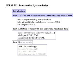
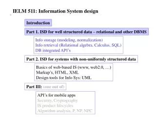
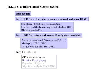
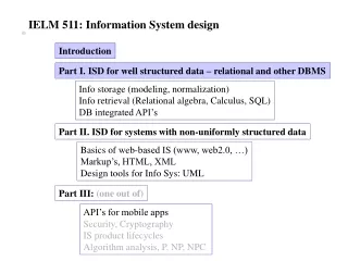
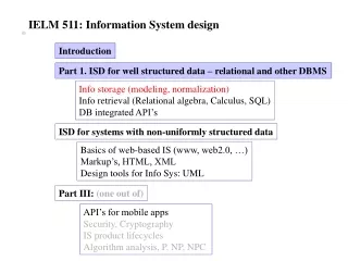
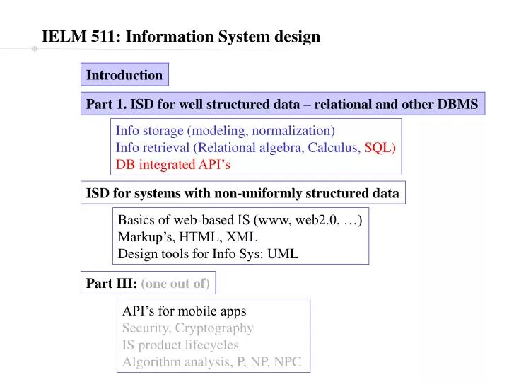
IELM 511: Information System design Introduction Part 1. ISD for well structured data – relational and other DBMS Info storage (modeling, normalization) Info retrieval (Relational algebra, Calculus, SQL) DB integrated API’s ISD for systems with non-uniformly structured data Basics of web-based IS (www, web2.0, …) Markup’s, HTML, XML Design tools for Info Sys: UML Part III: (one out of) API’s for mobile apps Security, Cryptography IS product lifecycles Algorithm analysis, P, NP, NPC

Agenda Structured Query Language (SQL) DB API’s

Recall our Bank DB design BRANCH( b_name, city, assets) CUSTOMER( cssn, c_name, street, city, banker, banker_type) LOAN( l_no, amount, br_name) PAYMENT(l_no, pay_no, date, amount) EMPLOYEE( e_ssn, e-name, tel, start_date, mgr_ssn) ACCOUNT( ac_no, balance) SACCOUNT( ac_no, int_rate) CACCOUNT( ac_no, od_amt) BORROWS(cust_ssn, loan_num) DEPOSIT(c_ssn, ac_num, access_date) DEPENDENT(emp_ssn, dep_name)

Background: Structured Query Language Basics of SQL: A DataBase Management System is an IT system Core requirements: - A structured way to store the definition of data [why ?]  DDL - Manipulation of data [obviously!]  DML SQL: a combined DDL+DML

SQL as a DDL A critical element of any design is to store the definitions of its components. In DB design, we deal with tables, using table names, attribute names etc. Each of these terms should have unambiguous syntax and semantics. A systematic way to specify and store these meta-data is by the use of a Data Definition Language The information about the data is stored in a Data Dictionary SQL provides a unified DDL + a Data Manipulation Language (DML).

SQL as a DDL: create command A DB stores one or more tables and one or more indexes To create a new database: createdatabase my_database; To create a new table: createtable my_table ( attribute_name attribute_type constraint, …., constraint, … ); A table stores data To create an index on a table: createindex my_index on my_table( attribute); An index is a special file for faster DB look-up, when searching the specified table for some data using the specified attribute.

SQL as a DDL: create command examples createdatabase bank; LOAN( l_no, amount, br_name) createtable loan ( l_no char(10), amount double, br_name char(30) references branch(b_name), primary key (loan_number) ); BORROWS(cust_ssn, loan_num) createtable borrows ( cust_ssn char(11), loan_num char(10), primary key (cust_ssn, loan_num), constraint borrows_c1 foreignkey cust_ssn references customer( cssn), constraint borrows_c2 foreignkey loan_num references loan( l_no) );

Note on metadata: system catalogs Metadata = data about data. DBMS manages a ‘data dictionary’ sometimes called ‘system catalog’ with - When was the DB and each table created/modified - Name of each attribute, its data type, and comments describing it, - List of all users who can access the DB and their passwords, - Which user can do what (read/add/update/delete/authorize) to the data. System catalog itself is stored in a table, and users can see (if they have authority) the data in it.

SQL as a DML: insert, drop commands To add one row into a table: insert into branch values( “Downtown”, “Brooklyn”, 9000000); insert into loan values( “L17”, 1000, “Downtown”); Note: char( ), date, datetime types: data must be “quoted” integer, single, double (number data types) are not quoted. Sequence in which you execute ‘insert’ matters ! This insert will fail unless table ‘branch’ has a row with ‘Downtown’ To remove an entire table from the DB: droptable branch; Note: this ‘drop’ command will fail if, e.g. there is data in table ‘loan’ [why?]

SQL as a DML: select command To get some data from a ( set of ) table (s): select attribute1, …, attribute_n from table_1, …, table_m where selection_or_join_condition1, …, selection_or_join_condition_r groupby attribute_i having aggregate_function( attribute_j, … ) orderby attribute_k Required Optional

SQL as a DML: select command To get some data from a ( set of ) table (s) select customer, loan_no from borrows; select * from borrows; select customer as “customer ssn” from borrows; select distinct loan_no from borrows; Notes: * is a wildcard as: gives alias name to attribute

SQL select: row filters Example: Find the names of all branches that have given loans larger than 1200 LOAN select distinct branch_name from loan where amount > 1200 Note: all operations in ‘where’ are applied one row at a time

SQL select: joins Example: Find the customer ssn, loan no, amount and branch name for all loans > 1200 select customer, loan.* from borrows, loan where loan_no = loan_number and amount > 1200 q-condition for join of loan, borrows selection condition WHERE clause: multiple q-conditions  and, or, not comparing cell values: >, =, !=, <, etc.

SQL select: joins with table and column aliases Example: Find the names of employees and their manager. select E.e_name as worker, M.e_name as boss from employee as E, employee as M where E.mgr_ssn = M.e_ssn Note: E, M are aliases (copies) of employee table

SQL select: nested queries, in Example: Find ssn of customers who have both deposit and loan select c_ssn from deposit where c_ssn in ( select customer from borrows) Notes: ‘in’ performs a set membership test

SQL select: nested queries, in Example: Find ssn of customers who have a deposit but no loan select c_ssn from deposit where c_ssn notin ( select customer from borrows) Notes: ‘not in’ is true if ‘in’ is false.

SQL select: nested, correlated queries, exists Existential qualifier (a generalization of ‘in’) Example: Find the names of branches that have given no loan select branch_name from branch where not exists ( select * from loan where branch.branch_name = loan.branch_name) 1. Correlated: ‘where’ clause of inner query refers to outer query 2. ‘exists’ is true is there is >= 1 row in evaluating inner query; ‘not exists’ is true is ‘exists’ is false

SQL select: arithmetic operations on columns Report the branch name and assets in units of millions select branch_name, assets*0.000001 as “assets (m)” from branch Notes: arithmetic ops can be used in SELECT, WHERE, HAVING

SQL select: group by, group-wise aggregation functions Example: Report the average, maximum amount, and number of loans by branch select branch_name, avg( amount) as Avg, max( amount) as Max, count( branch_name) as no_loans from loan groupby branch_name order by no_loans desc 1. Aggregating functions: avg, max, min, sum, count 2. avg/max return average/max for each group

SQL select: group by, having ‘having’ is used to screen out groups from the output Example: Report the small loans (<= 1500) held by 2 or more people. select loan_number, amount, count( loan_number) as no_debtors from loan, borrows where loan_number = loan_no and amount <= 1500 group by loan_number having count(loan_number) >= 2 ‘having’ conditions are only applied to data after rows have been grouped ‘order by’ used with ‘group by’ will be applied to groups.

SQL select: date functions SQL provides special functions to handle dates, times and strings Example: report those customers who have been inactive for over 5 years select c_ssn from deposit wheredatediff( yy, accessDate, getdate( ) ) > 5 datediff units: yy (years), …, ns (nano-seconds)

SQL select: string functions It is often useful to use wild-cards for string matching select ssn, name, street, city from customer where name LIKE ‘J%’ or street LIKE ‘[^mnp]%’ or city LIKE ‘%[ ]%’ Wildcards: %  zero or more chars [asd]  match one char out of list [asd] [^asd]  matches any one char except a, s, d.

SQL as a DML: update command… To modify an entry in a cell update loan set amount = amount - 200 where loan_number = ( select loan_no from borrows, customer where customer = ssn and name = ‘Jones’ ) select * from loan

SQL as a DML: delete command… To delete a row from a table delete from loan all rows of loan table deleted delete from customer where name = ‘Jones’ request to delete row of customer table with name = ‘Jones’ [will it succeed ?]

Views in SQL A view is a virtual table defined on a given Database: The columns of the view are either (i) columns from some (actual or virtual) table of the DB or (ii) columns that are computed (from other columns) Main uses of a view: - Security (selective display of information to different users) - Ease-of-use -- Explicit display of derived attributes -- Explicit display of related information from different tables -- Intermediate table can be used to simplify SQL query

Views in SQL.. Create a view showing the names of employees, their ssn, telephone number, their manager's name, and how many years they have worked in the bank. create view bank_employee as select e.e_ssn as ssn, e.e-name as name, e.tel as phone, m.e-name as manager, datediff( yy, start_date, getdate( )) as n_years from EMPLOYEE as e, EMPLOYEE as m where e.mgr_ssn = m.e_ssn select * from bank_employee

Operations on Views View definition is persistent – once you define it, the definition stays permanently in the DB until you drop the view. The DBMS only computes the data in a view when it is referenced in a SQL command (e.g. in a select … command) no physical table is stored in the stored memory corresponding to the view. You can use the view in any SQL query just the same as any other table, BUT (1) You cannot modify the value of a computed attribute (2) If an update/delete command is execute, the underlying data in the referenced table of the view is updated/deleted. [this can cause unexpected changes in your DB]

Concluding remarks on SQL SQL language has some other useful commands and operators [e.g. see here] In addition, most DBMS will provide many non-standard operators and services to facilitate information system deployment and administration. DBMSs can handle very large amount of data, and process queries very fast. IBM’s DB2 can handle over 6m transactions per min (tpm); Oracle 10g, over 4m tpm To speed up queries, you can use indexes. Common DBMSs: IBM DB2, Oracle 10g, Microsoft SQL Server, Sybase, MySQL. all support SQL.

DBMS DB your code odbc func more code SQL query odbc (DLL) Response Client App Database API’s Most people use DBs, but always through some computer program interface (API). Most DBMSs will provide program ‘libraries’ (a collection of a set of complied functions) with functions to: - Connect to the DBMS - Select a DB - Send a SQL command, and receive the response in some standard data structure. Each DBMS provides one library for each programming language. On Windows™ (and several other) systems, these libraries are called ODBC

Bank tables.. BRANCH EMPLOYEE

CUSTOMER DEPOSIT BORROWS LOAN Not all tables of our normalized design are shown; please create and populate for practice.

References and Further Reading Silberschatz, Korth, Sudarshan, Database Systems Concepts, McGraw Hill Next: IS for non-structured data

IELM 511: Information System design