Download
1 / 65
770 likes | 1.12k Vues
Food Shortages. Julianna Brunini Natalia Paine Danny Wilson. Context: population growth drives demand for food. World Population v. Time (1950-2100) Constant fertility High Medium Low. ← Nonlinear increase in meat consumption with increasing GDP.

E N D
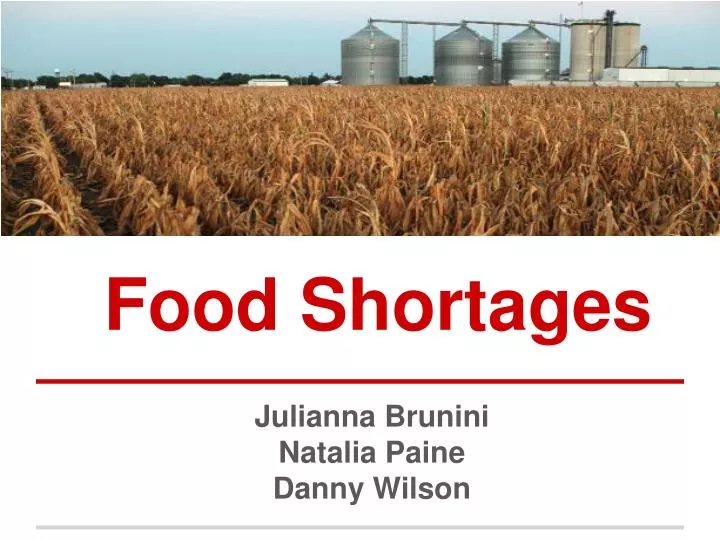
Food Shortages Julianna Brunini Natalia Paine Danny Wilson
Context: population growth drives demand for food World Population v. Time (1950-2100) Constant fertility High Medium Low ← Nonlinear increase in meat consumption with increasing GDP Production from Poultry and Pigs in China (1967-2007) Eggs Pigs Poultry Over 7 billion humans now live on the planet, consuming more crops and meat than ever before Million tonnes Images: Population Division of the UN, World Population Prospects: the 2012 Revision; Food and Agricultural Organization of the UN, Livestock and global food security, 2011
Worldwide famine has not yet ensued, thanks to technological innovation Farmer selection increases maize ear size The Green Revolution (1940s-1960s) spread fertilizers, pesticides, high-yield and dwarf cultivars throughout the developed and developing worlds. Norman Borlaug won the Nobel Peace Prize for his work on high-yield and dwarf cultivars Images: 1. Robert S. Peabody Museum of Archaeology, Phillips Academy, Andover, Massachusetts. 2. http://www.nytimes.com/2009/09/14/business/energy-environment/14borlaug.html?pagewanted=all&_r=0
Contemporary concern: maintaining food security as the climate changes Climatic factors that affect the food supply include precipitation, temperature and concentration of atmospheric gases Heat Waves ^ Temperature predictions under various emissions scenarios Desertification Storms and floods Images: Dole et. al (2011); IPCC 2013; environment.nationalgeographic.com; www.nrcs.usda.gov; IPCC
Today’s topic: how will increasing temperatures affect crop yields? Corn growth and Temperature Historical Temperature Exposure for US Corn (1950-2008): 35 C 5 C Temperatures outside the survival range injure crops. ← Growth range limits → www.extension.purdue.edu Images: Schlenker and Roberts (2009) Supplement; www.purdue.edu
In particular, we focus on crop yields and temperature in the eastern US 1. Soy Production by County, 2008 [Scale: 0 - 50+ bushels/acre] 2. Cotton Production by County, 2012 [Scale: 0-50+pounds/acre] 3.Corn Production by County, 2010 [Scale: 1 million - 20+ million bushels] 1 Schklenker & Roberts, Butler & Huybers 3 2 Images: USDA
Background: yield and agricultural output Yield (or agricultural output): • Quite simply: dry volume of crop produced per unit area of land cultivation • In the US, it’s measured in bushels/acre • Yield has a complex relationship with temperature Green Revolution Corn Yield in the US (1866-2012) Bushels per Acre
Before we begin: A “Bushel” and an “Acre” in Relatable Terms 1 acre is approximately ¾ the area of a football field Harvard Yard is about 10 acres
Review: regression models Purpose • To test the validity or falsity of a hypothesis The dependent variable is functionally related to the independent variable Yield Method: least-squares regression • Define “error” as the distance between the observation and the model prediction • Square the error terms to eliminate negative values • Minimize the sum of the squared errors Temp Data point Linear regression model Error = observed(x) - predicted(x)
Schlenker & Roberts aggregate corn, soy and cotton exposure to 1 degree C intervals from 1950-2005 across 2,000 US counties USDA Yield Data Weather data manipulated to “fine-scale” Home Weather Station http://www.nass.usda.gov/Charts_and_Maps/Crops_County/pdf/CR-PL12-RGBChor.pdf Schlenker (2006),Nonlinear effects of weather on cornfields
Schlenker and Roberts use an additive model, assuming yields are cumulative and proportional to temperature exposure yit = log(yield) in county i, year t g(h) = yield growth h = heat φit(h) = time distribution of heat zit = control factor (to account for technological change, precipitation) ci = fixed-county effect (to control for soil type, quality) Residual error upper temperature bound lower temperature bound
Histogram of Temperature Data for an average Corn Growing Season Histogram combines spatial and temporal data: - 50 growing seasons and 2000 counties - Normalized to the length of one growing season - Plotted as a histogram (x-axis is Temperature; y-axis is average number of days exposed to that particular one degree). In the model, the temperature distribution = φit(h) Threshold Temperature
Corn Shows Nonlinear Relationship between Temperature and Yield Note that the y-axis is logarithmic For corn, yield increases up to a threshold temperature (29 degrees C) and then drops precipitously. Threshold temperature Blue fit: step function Black fit: 8th-order polynomial Red fit: piecewise linear Anomaly of Log Yield (bushels) Exposure (days) ← Growth range limits → Temperature (Celsius) Schlenker and Roberts (2009), Figure 1
Understanding the Y-Axis - Anomaly of Log Yield (Bushels) - Misleadingly labeled Log Yield (Bushels) - A change of .01 on the axis corresponds to a 1% change in yield - A .075 decrease along the axis corresponds to a 7.5% decrease in yield Corn Anomaly of Log Yield (Bushels) Temperature (C)
Soy and Cotton Also Show Nonlinear Relationship between Temperature and Yield Soy Cotton For soy and cotton, the threshold temperatures are 30 and 32 degrees C, respectively. Schlenker and Roberts (2009), Figure 1 Anomaly of Log Yield (bushels) Temperature (Celsius) Temperature (Celsius) Threshold temperature
Schlenker and Roberts claim best out-of-sample predictions yet 56 years of data → Randomly choose 48 years and generate model estimates → Use model estimates to predict yields for the 8 leftover years Percent reduction in Root-Mean-Squared prediction error for various models Schlenker and Roberts (2009), Fig. 3 Compared to other models from the literature, Schlenker and Roberts’ reduces the root-mean-squared prediction error the most. Schlenker & Roberts models Other models
Schlenker and Roberts compare their model to three previous models Mendelsohn et al: Temperatures for January, April, July, October Deschenes et al: Daily mean temperatures to GDDs Schlenker et al: Thom’s relationship for daily temperature to monthly Previous predictions inferior because temperatures were averaged over time or space
Combining their statistical model with temperature forecasts, Schlenker and Roberts predict yield declines for 2070-2099 Colors match Figure 1 Blue = step function Black = 8th-order polynomial Red = piecewise linear Greater warming The authors predict 30-40% yield decreases under the slowest warming scenario; 63-82% decreases under the fastest warming scenario. Corn Soy Cotton Impacts by 2070-2099 (percent) Schlenker and Roberts (2009), Figure 2
Conclusions Persist Within Subsets of the Data The authors further divide the corn data by: • Temperature • Warmest, intermediate, and coldest regions • Time period • (1950-1977) and (1978-2005) • Level of precipitation • Quartiles of total rainfall during June and July • Alternative growing seasons For all subsets of the data, the authors observe a nonlinear trend between yield and temperature.
Breaking the dataset into warm, medium and cool subsets still results in a nonlinear trend between Yield and Temperature Corn—North The Northern subset shows a slightly higher threshold temperature and a steeper decline than the Southern subset. Anomaly of Log Yield (bushels) Corn—South Images: Schlenker and Roberts (2009) Supplementary Material
Breaking the data into an early period and a late period still results in a consistent, nonlinear trend between yield and temperature Soybeans (1950-1977) Soybeans (1977-2008) Average yields were greater between 1977 and 2008 than between 1950 and 1977, but the trend between yield and temperature is similar. Anomaly of Log Yield (bushels)
Precipitation quartiles show the same nonlinear trend between temperature and yield shown by the full dataset Corn: linear fit Corn: polynomial fit For corn, greater precipitation results in a shallower decline after the threshold temperature. Anomaly of Log Yield (bushels) Corn: step function fit
Choosing alternate growing seasons results in the same nonlinear relationship between yield and temperature Corn (April to August) Corn (March to September) Anomaly of Log Yield (bushels) Exposure (days) Exposure (days) Temperature (Celsius) Temperature (Celsius) For both extended and shortened growing seasons the nonlinear trend persists.
Schlenker & Roberts: Methods and Conclusions Method • Statistical regression, holding current growing regions fixed Conclusions • Non-linear trend: yields increase with temperature up to a threshold, above which they decline precipitously • Total yields decrease rapidly by 2099 for each of the 4 climate scenarios Fig. 1: Nonlinear relation between temperature and corn yield
Capacity for Agricultural Mobility within the United States and North America As temperatures rise, land suitable for growing will see a northward shift. S&R models hold current growing regions fixed.
Multiple Linear Regression: A review Butler and Huybers use multiple linear regression to measure the effects of several factors on yield. Multiple linear regression helps us answer four types of question: • Is at least one of the predictors useful in predicting the response? • Are all predictors useful or just a subset? • How well does the model fit the data? • Given a set of predictors, what responses can we expect? Remember: adding additional variables can only increase R2 → you want a theoretical basis to justify their inclusion Least-squares regression still applies Y = β0 +β1X1 +β2X2 +···+βpXp+ ε
Background: agricultural terms Killing Degree Days • Days that are so hot that they hinder grain development • KDD = sum of all all days with average temperatures greater than 29 degrees C (84 F) Growing Degree Days • Warm days that enable grain development • GDD = sum of all days with average temperatures greater than 8 degrees C (46 F) http://www.purdue.edu
Butler and Huybers (2013) look at maize across 1600 counties in the eastern US between 1981 and 2008 534 Weather Stations give daily minimum and maximum temperatures USDA Yield Data gives maize yield from 19 states
Butler and Huybers represent county yields using a linear combination of Growing Degree Days and Killing Degree Days Y = yield in county i t = technological change GDD = Growing Degree Days KDD = Killing Degree Days Epsilon = error Beta(0) = mean yield in county i (1951-2008) Beta(1) = sensitivity to technological change Beta(2) = cultivar sensitivity to growing degree days in county i Beta(3) = sensitivity to killing degree days in county i
Yield sensitivity to Growing Degree Days varies spatially Yield Sensitivity to GDDs (Beta-2) GDDs are a positive force on growth – they indicate higher yields In cooler regions, sensitivity to GDDs is 0.15 bushels/acre of yield Black boxes indicate irrigated counties Latitude Sensitivity to GDDs decreases in hotter regions Yield per GDD (0.00 - 0.16) Butler and Huybers (2013), Fig. 1a
Yield sensitivity to KDDs varies spatially, with lower sensitivity in hotter climates Yield Sensitivity to KDDs (Beta-3) Remember that KDDs → decreased yield Maize is from the tropics: adaptation interventions have been made for cold weather maize The authors take the spatial variation in KDD sensitivity as evidence of farmer adaptation Latitude Yield per KDD (-0.5 - 0.0) Butler and Huybers (2013), Fig. 1b
Distinguishing sensitivity from adaptation Sensitivity Strength of response to a given forcing Adaptation Actively choosing to minimize sensitivity to a particular forcing Sensitivity is a property of the plant, while adaptation refers to farming decisions http://farmindustrynews.com/corn-hybrids/purdue-gets-11-million-improve-heat-stress-tolerance-maize
Representing adapation: Butler and Huybers find a logarithmic relation between KDD sensitivity and climatology in unirrigated crops Red: logarithmic fit Red dashes: 95% confidence intervals Grey: linear and inverse fits Cold counties are most susceptible to yield loss from heat stress. Sensitivity (Bushels/ acre/KDD) Climatology (Mean KDD) Figure 2, Butler and Huybers (2013).
Incorporating adaptation into the model - Equation (1) describescounty Yield as a function of GDDs and KDDs - NO ADAPTATION YET • Spatial variation in Beta-3 is taken as evidence of adaptation • Logarithmic relation between KDD sensitivity and climatologyrepresents adaptation mathematically - The authors substitute (2) into (1) - Add 2 degrees C to all Ts - Fit Beta-3 for higher Ts - Calculate new yields using Beta-3 as a function of KDDs and higher temperatures Y = yield t = technological changes GDD = growing degree days KDD = killing degree days Beta-0: mean county yield Beta 1, 2, 3: sensitivity parameters Epsilon: residual error
Model output for 2 degree C warming: predicted yield losseswith (right) and without (left) adaptation Using equation 1 (no adaptation) Using equation 3 (with adaptation) When adaptation is included, predicted yield loss with 2 degree Celsius warming decreases from 14% to 6%. Yield increases in colder counties due to GDDs Yield decreases in hot counties due to KDDs Figure 3a, 3b Huybers and Butler (2013)
Schlenker and Roberts: adaptation does not ease the predicted impact of rising temperatures Blue, Black, Red represent no adaptation; Teal, Grey, Pink represent all farmers choosing to grow Southern corn. Impacts by 2020-2049, 2070-2099 (%)
Butler’s response: Schlenker’s data is heavily weighted by Southern counties Spatial → Variation in Yield Loss, generated by Butler using Schlenker and Robert’s modeling technique Yield losses occur in the South, while gains occur in the North The overall transfer function used by S&R is heavily determined by the South, biasing the results to favor greater losses
Schlenker: Butler’s approach to modeling adaptation is flawed Butler incorporates adaptation by making KDD sensitivity a function of climatology Schlenker argues that adaptation should alter all parameters, including the intercept and GDD sensitivity
Butler: we did look at GDD sensitivity and found it to be less important than KDD sensitivity Focus on GDD sensitivity… Even with GDD sensitivity included, losses within confidence interval Butler & Huybers, Figure S7
The debate: Where does adaptation come from? Which is it?
Butler cites previous work showing Southern resiliency Damage to Southern, Northern and Central Pioneer Hi-Bred Seeds Ristic (1996): “Southern hybrids displayed greater ability to withstand drought and heat stress conditions than central and northern hybrids.” → greater ability to synthesize heat stress proteins than northern hybrids Ristic et al (1996), Dehydration, damage to cellular membranes,and heat-shock proteins in maize hybrids from different climates
APPENDIX 43. Malthus 44. GMOs 45. Simulation models v. regression models 46-50. Regression example 51. Schlenker & Roberts paper flow 52. Linear v. Log scale 53. Agronomists v. economists 54. Climate models 55. Multiple linear regression example 56. Canada and farming migration northwards 58-61. Butler: what’s left out of the model 62-63. Stages of corn growth, most vulnerable stages of corn growth 64. Butler and Huybers v. Schlenker and Roberts
Context: a familiar dilemma? Thomas Malthus in the 18th century Malthus was concerned that exponential population growth would outpace linear growth in food production Images: http://www.lawbookexchange.com/images/44869.JPG; Image: http://wps.aw.com/aw_miller_econtoday_13/29/7556/1 934428.cw/content/index.html
In the 1970s, techniques emerged to genetically modify organisms; this process is fundamentally different from selective breeding To create GMOs, engineers take a desirable gene from one species and place it in the genome of another species Examples: • Insect immunity (Bt corn) • Vitamin A production (golden rice) Image: www.precisionnutrition.com
Background: mathematical models and agriculture Regression models Simulation models ← Scatterplot showing Grain Yield v. Total Above Ground Dry Matter Simulation model for maize → Simulated maize = green line Red dots = experimental data A strength of simulation models is that they utilize plant-growth theory; weaknesses include their complexity and oversight of farmers’ decisions. Regression models are able to incorporate farmers’ decisions, but they are susceptible to omitted variable bias. Images: http://www.ercim.eu/publication/Ercim_News/enw61/cournede.html; http://www.fao.org/docrep/w5183e/w5183e0e.htm
Regression primer: Boston dataset There are 14 variables examined, including crime rate per capita per town, tax rates, and distance to employment centers. There are 506 neighborhoods around Boston examined. The Boston dataset examines housing values in suburbs of Boston.
Boston dataset: Single linear regression – the basics Take median value (medv) as response with lower status of the population (lstat) as predictor In a single linear regression, our aim is to construct an equation that looks like this: Y ≈ β0 + β1X
Boston dataset: Single linear regression – key terms Here, we are regressing medv onto lstat. What does this mean? We must use the data we do have (training data) to estimate the coefficients. We use the least squares criterion to ensure that the line we generate is close to our data points When we run this in the statistical software R, we get: Intercept (B0) = 34.55 lstat (B1) = -0.95
Boston dataset: Single linear regression – the error term A more accurate representation of the linear regression equation is: Y = β0 + β1X + ε The additional term accounts for error. The model cannot account for everything: the relationship is probably not linear; variation in Y (or in this case, median value) is not controlled solely by X.
Boston dataset: Least squares regression line Median value (thousands of $) Lower status of the population