Download
1 / 52
540 likes | 783 Vues
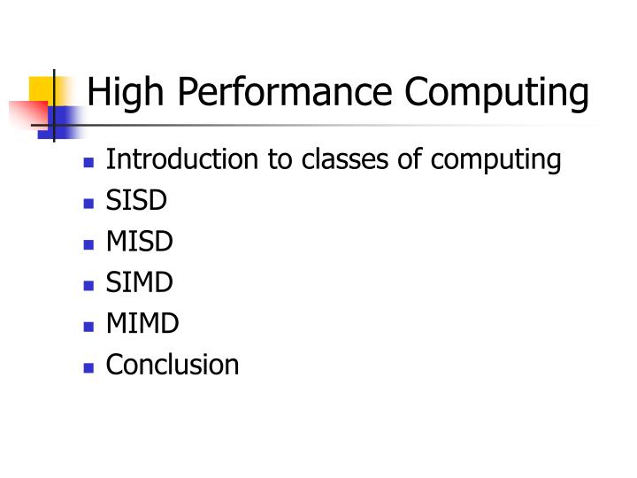
High Performance Computing. Introduction to classes of computing SISD MISD SIMD MIMD Conclusion. Classes of computing. Computation Consists of : Sequential Instructions (operation) Sequential dataset We can then abstractly classify into following classes of computing

E N D
High Performance Computing • Introduction to classes of computing • SISD • MISD • SIMD • MIMD • Conclusion
Classes of computing Computation Consists of : • Sequential Instructions (operation) • Sequential dataset We can then abstractly classify into following classes of computing system base on their characteristic instructions and dataset: • SISD Single Instruction, Single data • SIMD Single Instruction, Multiple data • MISD Multiple Instructions, Single data • MIMD Multiple Instructions, Multiple data
High Performance Computing • Introduction to classes of computing • SISD • MISD • SIMD • MIMD • Conclusion
SISD • Single Instruction Single Data • One stream of instruction • One stream of data • Scalar pipeline • To utilize CPU in most of the time • Super scalar pipeline • Increase the throughput • Expecting to increase CPI > 1 • Improvement from increase the “operation frequency”
SISD Example A = A + 1 Assemble code asm( “mov %%eax,%1 add $1,%eax :(=m) A”);
SISD Bottleneck • Level of Parallelism is low • Data dependency • Control dependency • Limitation improvements • Pipeline • Super scalar • Super-pipeline scalar
High Performance Computing • Introduction to classes of computing • SISD • MISD • SIMD • MIMD • Conclusion
MISD • Multiple Instructions Single Data • Multiple streams of instruction • Single stream of data • Multiple functionally unit operate on single data • Possible list of instructions or a complex instruction per operand (CISC) • Receive less attention compare to the other
MISD • Stream #1 Load R0,%1 Add $1,R0 Store R1,%1 • Stream #2 Load R0,%1 MUL %1,R0 Store R1,%1
MISD MISD ADD_MUL_SUB $1,$4,$7,%1 SISD Load R0,%1 ADD $1,R0 MUL $4,R0 STORE %1,R0
MISD bottleneck • Low level of parallelism • High synchronizations • High bandwidth required • CISC bottleneck • High complexity
High Performance Computing • Introduction to classes of computing • SISD • MISD • SIMD • MIMD • Conclusion
SIMD • Single Instruction, Multiple Data • Single Instruction stream • Multiple data streams • Each instruction operate on multiple data in parallel • Fine grained Level of Parallelism
SIMD • A wide variety of applications can be solved by parallel algorithms with SIMD • only problems that can be divided into sub problems, all of those can be solved simultaneously by the same set of instructions • This algorithms are typical easy to implement
SIMD • Example of • Ordinarily desktop and business applications • Word processor, database , OS and many more • Multimedia applications • 2D and 3D image processing, Game and etc • Scientific applications • CAD, Simulations
Example of CPU with SIMD ext • Intel P4 & AMD Althon, x86 CPU • 8 x 128 bits SIMD registers • G5 Vector CPU with SIMD extension • 32 x 128 bits registers • Playstation II • 2 vector units with SIMD extension
SIMD • SIMD instructions supports • Load and store • Integer • Floating point • Logical and Arithmetic instructions • Additional instruction (optional) • Cache instructions to support different locality for different type of application characteristic
Example of SIMD operation SIMD code Adding 2 sets of 4 32-bits integers V1 = {1,2,3,4} V2 = {5,5,5,5} VecLoad v0,%0 (ptr vector 1) VecLoad v1,%1 (ptr vector 2) VecAdd V1,V0 Or PMovdq mm0,%0 (ptr vector 1) PMovdq mm1,%1 (ptr vector 2) Paddwd mm1,mm0 Result V2 = {6,7,8,9}; Total instruction 2 load and 1 add Total of 3 instructions SISD code Adding 2 sets of 4 32-bits integers V1 = {1,2,3,4} V2 = {5,5,5,5} Push ecx (load counter register) Mov %eax,%0 (ptr vector Mov %ebx,%1 (ptr vector .LOOP Add %%ebx,%%eax (v2[i] = v1[i] + v2[i]) Add $4,%eax (v1++) Add $4,%ebx (v2++) Add $1,%eci (counter++) Branch counter < 4 Goto LOOP Result {6,7,8,9) Total instruction 3 Load + 4x (3 add) = 15 instructions SIMD
SIMD Matrix multiplication C code with Non-MMX int16 vect[Y_SIZE]; int16 matr[Y_SIZE][X_SIZE]; int16 result[X_SIZE]; int32 accum; for (i=0; i<X_SIZE; i++) { accum=0; for (j=0; j<Y_SIZE; j++) accum += vect[j]*matr[j][i]; result[i]=accum; }
SIMD Matrix multiplication C Code with MMX for (i=0; i<X_SIZE; i+=4) { accum = {0,0,0,0}; for (j=0; j<Y_SIZE; j+=2) accum += MULT4x2(&vect[j], &matr[j][i]); result[i..i+3] = accum; }
MULT4x2() • movd mm7, [esi] ; Load two elements from input vector • punpckldq mm7, mm7 ; Duplicate input vector: v0:v1:v0:v1 • movq mm0, [edx+0] ; Load first line of matrix (4 elements) • movq mm6, [edx+2*ecx] ; Load second line of matrix (4 elements) • movq mm1, mm0 ; Transpose matrix to column presentation punpcklwd mm0, mm6 ; mm0 keeps columns 0 and 1 • punpckhwd mm1, mm6 ; mm1 keeps columns 2 and 3 • pmaddwd mm0, mm7 ; multiply and add the 1st and 2nd column • pmaddwd mm1, mm7 ; multiply and add the 3rd and 4th column • paddd mm2, mm0 ; accumulate 32 bit results for col. 0/1 • paddd mm3, mm1 ; accumulate 32 bit results for col. 2/3
SIMD Matrix multiplication MMX with unrolled loop for (i=0; i<X_SIZE; i+=16) { accum={0,0,0,0,0,0,0,0,0,0,0,0,0,0,0,0}; for (j=0; j<Y_SIZE; j+=2) { accum[0..3] += MULT4x2(&vect[j], &matr[j][i]); accum[4..7] += MULT4x2(&vect[j], &matr[j][i+4]); accum[8..11] += MULT4x2(&vect[j], &matr[j][i+8]); accum[12..15] += MULT4x2(&vect[j], &matr[j][i+12]); } result[i..i+15] = accum; }
SIMD Matrix multiplication Source: Intel developer’s Matrix Multiply Application Note
SIMD MMX performance Source: http://www.tomshardware.com Article: Does the Pentium MMX Live up to the Expectations?
High Performance Computing • Introduction to classes of computing • SISD • MISD • SIMD • MIMD • Conclusion
MIMD • Multiple Instruction Multiple Data • Multiple streams of instructions • Multiple streams of data • Middle grained Parallelism level • Used to solve problem in parallel are those problems that lack the regular structure required by the SIMD model. • Implements in cluster or SMP systems • Each execution unit operate asynchronously on their own set of instructions and data, those could be a sub-problems of a single problem.
MIMD • Requires • Synchronization • Inter-process communications • Parallel algorithms • Those algorithms are difficult to design, analyze and implement
MPP Super-computer • High performance of single processor • Multi-processor MP • Cluster Network • Mixture of everything • Cluster of High performance MP nodes
Example of MPP Machines • Earth Simulator (2002) • Cray C90 • Cray X-MP
Cray X-MP • 1982 • 1 G flop • Multiprocessor with 2 or 4 Cray1-like processors • Shard memory
Cray C90 • 1992 • 1 G flop per processor • 8 or more processors
The Earth Simulator • Operational in late 2002 • Result of 5-year design and implementation effort • Equivalent power to top 15 US Machines
The Earth Simulator in details • 640 nodes • 8 vector processors per node, 5120 total • 8 G flops per processor, 40 T flops total • 16 GB memory per node, 10 TB total • 2800 km of cables • 320 cabinets (2 nodes each) • Cost: $ 350 million
High Performance Computing • Introduction to classes of computing • SISD • MISD • SIMD • MIMD • Conclusion
Conclusion • Massive Parallel Processing Age • Vector & SIMD 256 bits or even with 512 • MIMD • Parallel programming • Distribute programming • Quantum computing!!! • S/W slower than H/W development