Download
1 / 40
530 likes | 990 Vues
17. Consumption. 2 0 1 0 U P D A T E. This chapter covers:. an introduction to the most prominent work on consumption, including: John Maynard Keynes: consumption and current income Irving Fisher: intertemporal choice Franco Modigliani: the life-cycle hypothesis

E N D
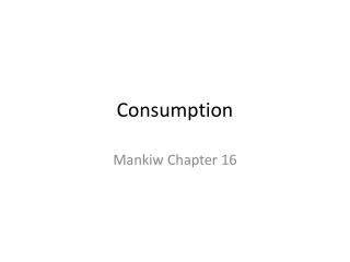
17 Consumption 2 0 1 0 U P D A T E
This chapter covers: an introduction to the most prominent work on consumption, including: John Maynard Keynes: consumption and current income Irving Fisher: intertemporal choice Franco Modigliani: the life-cycle hypothesis Milton Friedman: the permanent income hypothesis Robert Hall: the random-walk hypothesis (not covered) David Laibson: the pull of instant gratification(not covered)
Keynesian consumption function conjectures 1. 0 < MPC < 1 2. Average propensity to consume (APC) falls as income rises.(APC = C/Y ) 3. Income is the main determinant of consumption.
C c c = MPC = slope of the consumption function 1 Y The Keynesian consumption function
C slope = APC Y The Keynesian consumption function As income rises, consumers save a bigger fraction of their income, so APC falls.
Early empirical successes: Cross section and short time series results from early studies • Households with higher incomes: • consume more, MPC > 0 • save more, MPC < 1 • save a larger fraction of their income, APC as Y • Very strong correlation between income and consumption: income seemed to be the main determinant of consumption
Problems for the Keynesian consumption function • Based on the Keynesian consumption function, economists predicted that C would grow more slowly than Y over time. • This prediction did not come true: • As incomes grew, APC did not fall, and C grew at the same rate as income. • Simon Kuznets showed that C/Y was very stable in long time series data.
Consumption function from long time series data (constant APC ) C Consumption function from cross-sectional household data (falling APC ) Y The Consumption Puzzle
Irving Fisher and Intertemporal Choice • The basis for much subsequent work on consumption. • Assumes consumer is forward-looking and chooses consumption for the present and future to maximize lifetime satisfaction. • Consumer’s choices are subject to an intertemporal budget constraint, a measure of the total resources available for present and future consumption.
The basic two-period model • Period 1: the present • Period 2: the future • Notation Y1, Y2 = income in period 1, 2 C1, C2 = consumption in period 1, 2 S = Y1-C1 = saving in period 1 (S < 0 if the consumer borrows in period 1)
Period 2 budget constraint: Deriving the intertemporal budget constraint • Rearrange terms: • Divide through by (1+r) to get…
The intertemporal budget constraint present value of lifetime consumption present value of lifetime income
The budget constraint shows all combinations of C1 and C2 that just exhaust the consumer’s resources. C2 Consump = income in both periods Saving Y2 Borrowing C1 Y1 The intertemporal budget constraint
The slope of the budget line equals -(1+r ) 1 (1+r) Y2 Y1 The intertemporal budget constraint C2 C1
An indifference curve shows all combinations of C1 and C2that make the consumer equally happy. C2 IC2 IC1 C1 Consumer preferences Higher indifference curves represent higher levels of happiness.
Marginal rate of substitution (MRS): the amount of C2the consumer would be willing to substitute for one unit of C1. C2 1 MRS IC1 C1 Consumer preferences The slope of an indifference curve at any point equals the MRSat that point.
The optimal (C1,C2) is where the budget line just touches the highest indifference curve. C2 O C1 Optimization At the optimal point, MRS = 1+r
An increase in Y1 or Y2shifts the budget line outward. C2 C1 How C responds to changes in Y Results: Provided they are both normal goods, C1 and C2 both increase, …regardless of whether the income increase occurs in period 1 or period 2.
Keynes vs. Fisher • Keynes: Current consumption depends only on current income. • Fisher: Current consumption depends only on the present value of lifetime income. • The timing of income is irrelevant because the consumer can borrow or lend between periods.
An increase in r pivots the budget line around the point (Y1,Y2). C2 B A A Y2 C1 Y1 How C responds to changes in r As depicted here, C1 falls and C2 rises. However, it could turn out differently…
How C responds to changes in r • income effect: If consumer is a saver, the rise in r makes him better off, which tends to increase consumption in both periods. • substitution effect: The rise in r increases the opportunity cost of current consumption, which tends to reduce C1 and increase C2. • Both effects C2. Whether C1 rises or falls depends on the relative size of the income & substitution effects.
Constraints on borrowing • In Fisher’s theory, the timing of income is irrelevant: Consumer can borrow and lend across periods. • Example: If consumer learns that her future income will increase, she can spread the extra consumption over both periods by borrowing in the current period. • However, if consumer faces borrowing constraints (aka “liquidity constraints”), then she may not be able to increase current consumption …and her consumption may behave as in the Keynesian theory even though she is rational & forward-looking.
The budget line with no borrowing constraints C2 C1 Constraints on borrowing Y2 Y1
The borrowing constraint takes the form: C1Y1 C2 The budget line with a borrowing constraint C1 Constraints on borrowing Y2 Y1
The borrowing constraint is not binding if the consumer’s optimal C1is less than Y1. C2 C1 Consumer optimization when the borrowing constraint is not binding Y1
The optimal choice is at point D. But since the consumer cannot borrow, the best he can do is point E. C2 C1 Consumer optimization when the borrowing constraint is binding E D Y1
The Life-Cycle Hypothesis • due to Franco Modigliani (1950s) • Fisher’s model says that consumption depends on lifetime income, and people try to achieve smooth consumption. • The LCH says that income varies systematically over the phases of the consumer’s “life cycle,” and saving allows the consumer to achieve smooth consumption.
The Life-Cycle Hypothesis • The basic model: W = initial wealth Y = annual income until retirement (assumed constant) R = number of years until retirement T = lifetime in years • Assumptions: • zero real interest rate (for simplicity) • consumption-smoothing is optimal
The Life-Cycle Hypothesis • Lifetime resources = W + RY • To achieve smooth consumption, consumer divides her resources equally over time: C = (W + RY )/T , or C = aW +bY where a = (1/T ) is the marginal propensity to consume out of wealth b = (R/T ) is the marginal propensity to consume out of income
Implications of the Life-Cycle Hypothesis The LCH can solve the consumption puzzle: • The life-cycle consumption function implies APC = C/Y = a(W/Y ) +b • Across households, income varies more than wealth, so high-income households should have a lower APC than low-income households. • Over time, aggregate wealth and income grow together, causing APC to remain stable.
The LCH implies that saving varies systematically over a person’s lifetime. $ Wealth Income Saving Consumption Dissaving Retirement begins End of life Implications of the Life-Cycle Hypothesis
The Permanent Income Hypothesis • due to Milton Friedman (1957) • Y = YP + YT where Y = current income YP = permanent incomeaverage income, which people expect to persist into the future YT = transitory incometemporary deviations from average income
The Permanent Income Hypothesis • Consumers use saving & borrowing to smooth consumption in response to transitory changes in income. • The PIH consumption function: C = aYP where a is the fraction of permanent income that people consume per year.
The Permanent Income Hypothesis The PIH can solve the consumption puzzle: • The PIH impliesAPC = C/Y = aYP/Y • If high-income households have higher transitory income than low-income households, APC is lower in high-income households. • Over the long run, income variation is due mainly (if not solely) to variation in permanent income, which implies a stable APC.
PIH vs. LCH • Both: people try to smooth their consumption in the face of changing current income. • LCH: current income changes systematically as people move through their life cycle. • PIH: current income is subject to random, transitory fluctuations. • Both can explain the consumption puzzle.
Summing up • Keynes: consumption depends primarily on current income. • Recent work: consumption also depends on • expected future income • wealth • interest rates • Economists disagree over the relative importance of these factors, borrowing constraints, and psychological factors.
Chapter Summary 1. Keynesian consumption theory Keynes’ conjectures MPC is between 0 and 1 APC falls as income rises current income is the main determinant of current consumption Empirical studies in household data & short time series: confirmation of Keynes’ conjectures in long-time series data:APC does not fall as income rises
Chapter Summary 2. Fisher’s theory of intertemporal choice Consumer chooses current & future consumption to maximize lifetime satisfaction of subject to an intertemporal budget constraint. Current consumption depends on lifetime income, not current income, provided consumer can borrow & save.
Chapter Summary 3. Modigliani’s life-cycle hypothesis Income varies systematically over a lifetime. Consumers use saving & borrowing to smooth consumption. Consumption depends on income & wealth.
Chapter Summary 4. Friedman’s permanent-income hypothesis Consumption depends mainly on permanent income. Consumers use saving & borrowing to smooth consumption in the face of transitory fluctuations in income.