Download
1 / 23
230 likes | 339 Vues
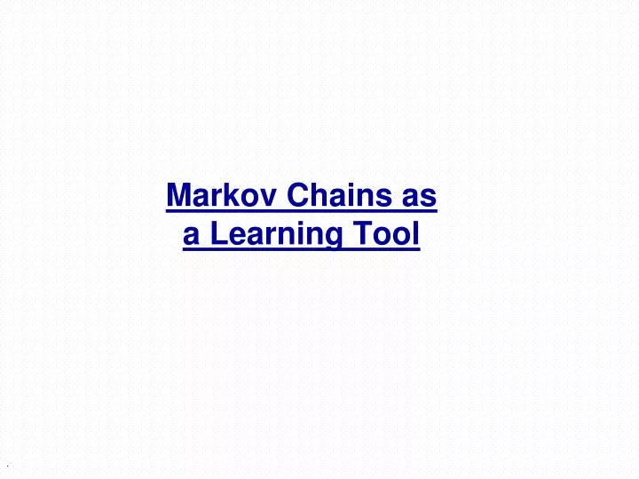
Markov Chains as a Learning Tool. 0.6. 0.4. 0.8. rain. no rain. 0.2. Markov Process Simple Example. Weather: raining today 40% rain tomorrow 60% no rain tomorrow not raining today 20% rain tomorrow 80% no rain tomorrow. Stochastic Finite State Machine:.

E N D
0.6 0.4 0.8 rain no rain 0.2 Markov ProcessSimple Example • Weather: • raining today 40% rain tomorrow • 60% no rain tomorrow • not raining today 20% rain tomorrow • 80% no rain tomorrow Stochastic Finite State Machine:
Markov ProcessSimple Example • Weather: • raining today 40% rain tomorrow • 60% no rain tomorrow • not raining today 20% rain tomorrow • 80% no rain tomorrow The transition matrix: • Stochastic matrix: • Rows sum up to 1 • Double stochastic matrix: • Rows and columns sum up to 1 Rain No rain Rain No rain
X2 X4 X3 X1 X5 Markov Process Let Xi be the weather of day i, 1 <= i <= t. We may decide the probability of Xt+1 from Xi, 1 <= i <= t. • Markov Property:Xt+1, the state of the system at time t+1 depends only on the state of the system at time t • Stationary Assumption:Transition probabilities are independent of time (t)
p p p p 0 1 99 2 100 Start (10$) 1-p 1-p 1-p 1-p Markov ProcessGambler’s Example • – Gambler starts with $10 (the initial state) • - At each play we have one of the following: • • Gambler wins $1 with probabilityp • • Gambler looses $1 with probability 1-p • – Game ends when gambler goes broke, or gains a fortune of $100 • (Both 0 and 100 are absorbing states) 1-p
p p p p 0 1 99 2 100 Start (10$) 1-p 1-p 1-p 1-p Markov Process • Markov process - described by a stochastic FSM • Markov chain - a random walk on this graph • (distribution over paths) • Edge-weights give us • We can ask more complex questions, like
0.1 0.9 0.8 coke pepsi 0.2 Markov ProcessCoke vs. Pepsi Example • Given that a person’s last cola purchase was Coke, there is a 90% chance that his next cola purchase will also be Coke. • If a person’s last cola purchase was Pepsi, there is an 80% chance that his next cola purchase will also be Pepsi. transition matrix: coke pepsi coke pepsi
Markov ProcessCoke vs. Pepsi Example (cont) Given that a person is currently a Pepsi purchaser, what is the probability that he will purchase Coke two purchases from now? Pr[ Pepsi?Coke ] = Pr[ PepsiCokeCoke ] +Pr[ Pepsi Pepsi Coke ] = 0.2 * 0.9 + 0.8 * 0.2 = 0.34 ? Coke Pepsi ?
Markov ProcessCoke vs. Pepsi Example (cont) Given that a person is currently a Coke purchaser, what is the probability that he will buy Pepsi at the third purchase from now?
Markov ProcessCoke vs. Pepsi Example (cont) • Assume each person makes one cola purchase per week • Suppose 60% of all people now drink Coke, and 40% drink Pepsi • What fraction of people will be drinking Coke three weeks from now? Pr[X3=Coke] = 0.6 * 0.781 + 0.4 * 0.438 = 0.6438 Qi- the distribution in week i Q0= (0.6,0.4) - initial distribution Q3= Q0 * P3 =(0.6438,0.3562)
stationary distribution 0.1 0.9 0.8 coke pepsi 0.2 Markov ProcessCoke vs. Pepsi Example (cont) Simulation: 2/3 Pr[Xi= Coke] week - i
How to obtain Stochastic matrix? • Solve the linear equations, e.g., • Learn from examples, e.g., what letters follow what letters in English words: mast, tame, same, teams, team, meat, steam, stem.
How to obtain Stochastic matrix? • Counts table vs Stochastic Matrix
Application of Stochastic matrix • Using Stochastic Matrix to generate a random word: • Generate most likely first letter • For each current letter generate most likely next letter C If C[r,j] > 0, let A[r,j] = C[r,1]+C[r,2]+…+C[r,j]
Application of Stochastic matrix • Using Stochastic Matrix to generate a random word: • Generate most likely first letter: Generate a random number x between 1 and 8. If 1 <= x <= 3, the letter is ‘s’; if 4 <= x <= 6, the letter is ‘t’; otherwise, it’s ‘m’. • For each current letter generate most likely next letter: Suppose the current letter is ‘s’ and we generate a random number x between 1 and 5. If x = 1, the next letter is ‘a’; if 2 <= x <= 4, the next letter is ‘t’; otherwise, the current letter is an ending letter. If C[r,j] > 0, let A[r,j] = C[r,1]+C[r,2]+…+C[r,j]
Supervised vs Unsupervised • Decision tree learning is “supervised learning” as we know the correct output of each example. • Learning based on Markov chains is “unsupervised learning” as we don’t know which is the correct output of “next letter”.
K-Nearest Neighbor • Features • All instances correspond to points in an n-dimensional Euclidean space • Classification is delayed till a new instance arrives • Classification done by comparing feature vectors of the different points • Target function may be discrete or real-valued
Example:Identify Animal Type 14 examples 10 attributes 5 types What’s the type of this new animal?
K-Nearest Neighbor • An arbitrary instance is represented by (a1(x), a2(x), a3(x),.., an(x)) • ai(x) denotes features • Euclidean distance between two instances d(xi, xj)=sqrt (sum for r=1 to n (ar(xi) - ar(xj))2) • Continuous valued target function • mean value of the k nearest training examples
Distance-Weighted Nearest Neighbor Algorithm • Assign weights to the neighbors based on their ‘distance’ from the query point • Weight ‘may’ be inverse square of the distances • All training points may influence a particular instance • Shepard’s method
Remarks + Highly effective inductive inference method for noisy training data and complex target functions + Target function for a whole space may be described as a combination of less complex local approximations + Learning is very simple - Classification is time consuming (except 1NN)